Factor analysis is one of the most powerful statistical data analysis tools. It is based on the procedure for combining groups of variables that correlate with each other (“correlation pleiades” or “correlation nodes”) into several factors.
In other words, the purpose of factor analysis is to concentrate the initial information, expressing a large number of considered features through a smaller number of more capacious internal characteristics, which, however, cannot be directly measured (and in this sense are latent).
For example, let's hypothetically imagine a legislature at the regional level, consisting of 100 deputies. Among the various issues on the agenda for voting are: a) a bill proposing to restore the monument to V.I. Lenin on the central square of the city - the administrative center of the region; b) an appeal to the President of the Russian Federation with a demand to return all strategic production to state ownership. The contingency matrix shows the following distribution of deputies' votes:
| Monument to Lenin (for) | Monument to Lenin (against) | |
| Appeal to the President (for) | 49 | 4 |
| Appeal to the President (against) | 6 | 41 |
Obviously, the votes are statistically related: the vast majority of deputies who support the idea of restoring the monument to Lenin also support the return to state ownership strategic enterprises. Similarly, most opponents of the restoration of the monument are at the same time opponents of the return of enterprises to state ownership. At the same time, the voting is completely unrelated to each other thematically.
It is logical to assume that the revealed statistical relationship is due to the existence of some hidden (latent) factor. Legislators, formulating their point of view on a wide variety of issues, are guided by a limited, small set of political positions. In this case, we can assume the presence of a hidden split in the deputies according to the criterion of support / rejection of conservative socialist values. A group of "conservatives" stands out (according to our contingency table - 49 deputies) and their opponents (41 deputies). Having identified such splits, we can describe a large number of individual votes in terms of a small number of factors that are latent in the sense that we cannot detect them directly: in our hypothetical parliament, there was never a vote in which MPs were asked to determine their attitude towards conservative socialist values. We detect the presence of this factor based on a meaningful analysis of quantitative relationships between variables. Moreover, if nominal variables are deliberately taken in our example - support for the bill with the categories “for” (1) and “against” (0), then in reality factor analysis effectively processes interval data.
Factor analysis is widely used in political science, and in "neighboring" sociology and psychology. One of the main reasons for the high demand this method consists in a variety of tasks that can be solved with its help. Thus, there are at least three “typical” goals of factor analysis:
dimensionality reduction (reduction) of data. Factor analysis, highlighting the nodes of interrelated features and reducing them to some generalized factors, reduces the initial basis of features of the description. The solution of this problem is important in a situation where objects are measured by a large number of variables and the researcher is looking for a way to group them according to a semantic feature. The transition from many variables to several factors makes it possible to make the description more compact, to get rid of uninformative and duplicate variables;
Revealing the structure of objects or features (classification). This problem is close to that which is solved by the cluster analysis method. But if cluster analysis takes their values for several variables as the “coordinates” of objects, then factor analysis determines the position of the object relative to factors (related groups of variables). In other words, with the help of factor analysis, one can evaluate the similarity and difference of objects in the space of their correlations, or in the factor space. The resulting latent variables act as the coordinate axes of the factor space, the objects under consideration are projected onto these axes, which makes it possible to create a visual geometric representation of the studied data, convenient for meaningful interpretation;
indirect measurement. Factors, being latent (empirically not observable), cannot be directly measured. However, factor analysis allows not only to identify latent variables, but also to quantify their value for each object.
Let us consider the algorithm and interpretation of the factor analysis statistics using the data on the results of the parliamentary elections in the Ryazan region in 1999 (a federal district) as an example. To simplify the example, let's take electoral statistics only for those parties that have overcome the 5% threshold. The data is taken in the context of territorial election commissions (by cities and districts of the region).
The first step is to standardize the data by converting it to standard scores (so-called L-scores calculated using the normal distribution function).
| TEAK (territorial election commission) | "Apple" | "Unity" | Block Zhirinovsky | OVR | CPRF | THX |
| Ermishinskaya | 1,49 | 35,19 | 6,12 | 5,35 | 31,41 | 2,80 |
| Zakharovskaya | 2,74 | 18,33 | 7,41 | 11,41 | 31,59 | l b 3" |
| Kadomskaya | 1,09 | 29,61 | 8,36 | 5,53 | 35,87 | 1,94 |
| Kasimovskaya | 1,30 | 39,56 | 5,92 | 5,28 | 29,96 | 2,37 |
| Kasimovskaya city | 3,28 | 39,41 | 5,65 | 6,14 | 24,66 | 4,61 |
| The same in standardized scores (g-scores) | ||||||
| Ermishinskaya | -0,83 | 1,58 | -0,25 | -0,91 | -0,17 | -0,74 |
| Zakharovskaya | -0,22 | -1,16 | 0,97 | 0,44 | -0,14 | 0,43 |
| Kadomskaya | -1,03 | 0,67 | 1,88 | -0,87 | 0,59 | -1,10 |
| Kasimovskaya | -0,93 | 2,29 | -0,44 | -0,92 | -0,42 | -0,92 |
| Kasimovskaya city | 0,04 | 2,26 | -0,70 | -0,73 | -1,32 | 0,01 |
| Etc. (total 32 cases) | ||||||
| "Apple" | "Unity" | BJ | OVR | CPRF | THX | |
| "Apple" | ||||||
| "Unity" | -0,55 | |||||
| BJ | -0,47 | 0,27 | ||||
| OVR | 0,60 | -0,72 | -0,47 | |||
| CPRF | -0,61 | 0,01 | 0,10 | -0,48 | ||
| THX | 0,94 | -0,45 | -0,39 | 0,52 | -0,67 |
Already a visual analysis of the matrix of pair correlations allows us to make assumptions about the composition and nature of the correlation pleiades. For example, positive correlations are found for the "Union of Right Forces", "Yabloko" and the "Fatherland - All Russia" bloc (pairs "Yabloko" - OVR, "Yabloko" - SPS and OVR - SPS). At the same time, these three variables are negatively correlated with the CPRF (support for the CPRF), to a lesser extent with Unity (support for Unity), and even less with the BZ variable (support for the Zhirinovsky Bloc). Thus, we presumably have two pronounced correlation pleiades:
("Yabloko" + OVR + SPS) - the Communist Party of the Russian Federation;
("Yabloko" + OVR + SPS) - "Unity".
These are two different pleiades, not one, since there is no connection between Unity and the Communist Party of the Russian Federation (0.01). As for the BZ variable, it is more difficult to make an assumption, here the correlations are less pronounced.
To test our assumptions, we need to CALCULATE the eigenvalues of the factors (eigenvalues), factor scores, and factor loadings for each variable. Such calculations are quite complicated and require serious skills in working with matrices, so we will not consider the computational aspect here. We will only say that these calculations can be carried out in two ways: the method of principal components (principal components) and the method of principal factors (principal factors). Principal component method is more common, statistical programs use it "by default".
Let us dwell on the interpretation of eigenvalues, factorial values and factor loadings.
The eigenvalues of the factors for our case are as follows:
| Factor | Eigenvalue | % total variation |
| 1 | 3,52 | 58,75 |
| 2 | 1,14 | 19,08 |
| 3 | 0,76 | 12,64 |
| 4 | 0,49 | S.22 |
| 0,05 | 0.80 | |
| 6 | 0,03 | 0,51 |
| Total | 6 | 100% |
The greater the eigenvalue of the factor, the greater its explanatory power (the maximum value is equal to the number of variables, in our case 6). One of the key elements of factor analysis statistics is the % total variance indicator. It shows what proportion of the variation (variability) of variables explains the extracted factor. In our case, the weight of the first factor outweighs the weight of all other factors combined: it explains almost 59% of the total variation. The second factor explains 19% of the variation, the third - 12.6%, and so on. descending.
Having the eigenvalues of the factors, we can start solving the problem of data dimension reduction. The reduction will occur due to the exclusion from the model of factors that have the least explanatory power. And here the key question is how many factors to leave in the model and what criteria to follow. So, factors 5 and 6 are clearly superfluous, which together explain a little more than 1% of the entire variation. But the fate of factors 3 and 4 is no longer so obvious.
As a rule, factors remain in the model, the eigenvalue of which exceeds unity (the Kaiser criterion). In our case, these are factors 1 and 2. However, it is useful to check the correctness of removing four factors using other criteria. One of the most widely used methods is scree plot analysis. For our case, it looks like:
The chart got its name from its resemblance to the side of a mountain. "Scree" is a geological term for debris rocks accumulating in the lower part of the rocky slope. "Rock" is truly influential factors, "scree" is statistical noise. Figuratively speaking, you need to find a place on the graph where the “rock” ends and the “scree” begins (where the decrease in eigenvalues from left to right is greatly slowed down). In our case, the choice must be made from the first and second inflections corresponding to two and four factors. Leaving four factors, we get a very high accuracy of the model (more than 98% of the total variation), but make it quite complex. Leaving two factors, we will have a significant unexplained part of the variation (about 22%), but the model will become concise and easy to analyze (in particular, visually). Thus, in this case, it is better to sacrifice some accuracy in favor of compactness, leaving the first and second factors.
You can check the adequacy of the obtained model using special matrices of reproduced correlations and residual coefficients (residual correlations). The matrix of reproduced correlations contains the coefficients that were recovered from the two factors left in the model. Of particular importance in it is the main diagonal, on which the commonalities of variables are located (in italics in the table), which show how accurately the model reproduces the correlation of a variable with the same variable, which should be unity.
The matrix of residual coefficients contains the difference between the original and reproduced coefficients. For example, the reproduced correlation between the ATP and Yabloko variables is 0.88, while the original one is 0.94. Remainder = 0.94 - 0.88 = 0.06. The lower the residual values, the higher the quality of the model.
| Reproduced correlations | ||||||
| "Apple" | "Unity" | BJ | OVR | CPRF | THX | |
| "Apple" | 0,89 | |||||
| "Unity" | -0,53 | 0,80 | ||||
| BJ | -0,47 | 0,59 | 0,44 | |||
| OVR | 0,73 | -0,72 | -0,56 | 0,76 | ||
| CPRF | -0,70 | 0,01 | 0,12 | -0,34 | 0,89 | |
| THX | 0,88 -0,43 | -0,40 | 0,66 | -0,77 | 0,88 | |
| Residual odds | ||||||
| "Apple" | "Unity" | BJ | OVR | CPRF | THX | |
| "Apple" | 0,11 | |||||
| "Unity" | -0,02 | 0,20 | ||||
| BJ | 0,00 | -0,31 | 0,56 | |||
| OVR | -0,13 | -0,01 | 0,09 | 0,24 | ||
| CPRF | 0,09 | 0,00 | -0,02 | -0,14 | 0,11 | |
| THX | 0,06 | -0,03 | 0,01 | -0,14 | 0,10 | 0,12 |
As can be seen from the matrices, the two-factor model, being generally adequate, does not explain individual relationships well. Thus, the generality of the BZ variable is very low (only 0.56), the value of the residual coefficient of connection between BZ and “Unity” is too high (-0.31).
Now it is necessary to decide how important an adequate representation of the BJ variable is for this particular study. If the importance is high (for example, if the study is devoted to the analysis of the electorate of this particular party), it is correct to return to the four-factor model. If not, two factors can be left.
Taking into account the educational nature of our tasks, we leave a simpler model.
Factor loads can be represented as correlation coefficients of each variable with each of the identified factors 1ak, the correlation between the values of the first factor variable and the values of the "Apple" variable is -0.93. All factor loadings are given in the factor mapping matrix-
The closer the relationship of the variable with the factor under consideration, the higher the value of the factor load. The positive sign of the factor load indicates a direct, and the negative sign indicates the feedback of the variable with the factor.
Having the values of factor loads, we can construct a geometric representation of the results of factor analysis. On the X axis, we plot the loads of variables on factor 1, on the Y axis, the loads of variables on factor 2, and we get a two-dimensional factor space.

Before proceeding to a meaningful analysis of the results obtained, let's perform one more operation - rotation. The importance of this operation is dictated by the fact that there is not one, but many variants of the matrix of factor loads that equally explain the relationships of variables (the matrix of intercorrelations). It is necessary to choose a solution that is easier to interpret meaningfully. This is considered a load matrix in which the values of each variable for each factor are maximized or minimized (close to one or zero).
Consider a schematic example. There are four objects located in the factor space as follows:
 |
Loads on both factors for all objects are significantly different from zero, and we are forced to use both factors to interpret the position of objects. But if we “rotate” the entire structure clockwise around the intersection of the coordinate axes, we get the following picture:
In this case, the loads on factor 1 will be close to zero, and the loads on factor 2 will be close to unity (simple structure principle). Accordingly, for a meaningful interpretation of the position of objects, we will involve only one factor - factor 2.
There are quite a number of methods for rotating factors. Thus, the group of orthogonal rotation methods always preserves a right angle between the coordinate axes. These include vanmax (minimizes the number of variables with a high factor load), quartimax (minimizes the number of factors needed to explain the variable), equamax (a combination of the two previous methods). Oblique rotation methods do not necessarily preserve a right angle between the axes (eg direct obiimin). The promax method is a combination of orthogonal and oblique rotation methods. In most cases, the vanmax method is used, which gives good results for most policy research tasks. Also, as with many other methods, it's a good idea to experiment with different rotation techniques.
In our example, after rotation by the varimax method, we obtain the following matrix of factor loadings:
Accordingly, the geometric representation of the factor space will look like:

Now we can proceed to a meaningful interpretation of the results obtained. The key opposition - the electoral split - according to the first factor is formed by the Communist Party of the Russian Federation on the one hand, and Yabloko and the Union of Right Forces (to a lesser extent OVR) - on the other. Substantially - based on the specifics of the ideological attitudes of the named subjects of the electoral process - we can interpret this demarcation as a "left-right" split, which is "classical" for political science.
Opposition on factor 2 is formed by OVR and Unity. The latter is adjoined by the “Zhirinovsky Block”, but we cannot reliably judge its position in the factor space due to the features of the model, which poorly explains the relationships of this particular variable. To explain this configuration, it is necessary to recall the political realities of the 1999 election campaign. At that time, the struggle within the political elite led to the formation of two echelons of the "party of power" - the "Unity" and "Fatherland - All Russia" blocs. The difference between them was not of an ideological nature: in fact, the population was offered to choose not from two ideological platforms, but from two elite groups, each of which had significant power resources and regional support. Thus, this split can be interpreted as "power-elite" (or, somewhat simplifying, "power-opposition").
In general, we get a geometric representation of a certain electoral space of the Ryazan region for these elections, if we understand the electoral space as a space of electoral choice, the structure of key political alternatives (“splits”). The combination of these two splits was very typical of the 1999 parliamentary elections.
Comparing the results of factor analysis for the same region in different elections, we can judge the presence of continuity in the configuration of the space of electoral choice of territory. For example, a factor analysis of the federal parliamentary elections (1995, 1999 and 2003) held in Tatarstan showed a stable configuration of the electoral space. For the 1999 elections, only one factor was left in the model with an explanatory power of 83% of the variation, which made it impossible to build a two-dimensional diagram. The corresponding column shows factor loadings.
If you look closely at these results, you will notice that in the republic, from election to election, the same main split is reproduced: ““ the party in power ”- all the rest.” "(NDR), in 1999 - OVR, in 2003 - "United Russia". Over time, only the "details" change - the name of the "party of power". The new political "label" very easily fits into the static matrix of a one-dimensional political choice.
At the end of the chapter, we will give one practical advice. The success of the development of statistical methods, by and large, is possible only with intensive practical work with special programs (the already mentioned SPSS, Statistica or at least Microsoft Excel). It is no coincidence that the presentation of statistical techniques is conducted by us in the mode of work algorithms: this allows the student to independently go through all the stages of analysis, sitting at the computer. Without attempts at practical analysis of real data, the idea of the possibilities of statistical methods in political analysis will inevitably remain general and abstract. And today the ability to apply statistics to solve both theoretical and applied problems is a fundamentally important component of the model of a political scientist.
Control questions and tasks
1. What levels of measurement correspond to the average values - mode, median, arithmetic mean? What measures of variation are typical for each of them?
2. For what reasons it is necessary to take into account the form of distribution of variables?
3. What does the statement “There is a statistical relationship between two variables” mean?
4. What useful information about relationships between variables can be obtained based on the analysis of contingency tables?
5. What can be learned about the relationship between variables based on the values of the chi-square and lambda statistical tests?
6. Define the concept of "error" in statistical research. How can this indicator be used to judge the quality of the constructed statistical model?
7. What is the main purpose of correlation analysis? What characteristics of a statistical relationship does this method reveal?
8. How to interpret the value of the Pearson correlation coefficient?
9. Describe the method of dispersion analysis. What other statistical methods use ANOVA statistics and why?
10. Explain the meaning of the term "null hypothesis".
11. What is a regression line, what method is used to build it?
12. What does the coefficient R show in the final statistics of the regression analysis?
13. Explain the term "multidimensional classification method".
14. Explain the main differences between clustering using hierarchical cluster analysis and K-means.
15. How can cluster analysis be used to study the image of political leaders?
16. What is the main task solved by discriminant analysis? Define a discriminant function.
17. Name three classes of problems solved using factor analysis. Define the term "factor".
18. Describe the three main methods for checking the quality of the model in factor analysis (Kaiser's criterion, the "scree" criterion, the matrix of reproduced correlations).
All processes in business are interconnected. There are both direct and indirect links between them. Various economic parameters change under the influence of various factors. Factor analysis (FA) allows you to identify these indicators, analyze them, and study the degree of influence.
The concept of factor analysis
Factor analysis is a multivariate technique that allows you to study the relationship between the parameters of variables. In the process, the structure of covariance or correlation matrices is studied. Factor analysis is used in a variety of sciences: psychometrics, psychology, economics. The basics of this method were developed by psychologist F. Galton.
Tasks
To obtain reliable results, a person needs to compare indicators on several scales. In the process, the correlation of the obtained values, their similarities and differences are determined. Consider the basic tasks of factor analysis:
- Detection of existing values.
- Selection of parameters for a complete analysis of values.
- Classification of indicators for system work.
- Detection of interrelations between effective and factorial values.
- Determining the degree of influence of each of the factors.
- Analysis of the role of each of the values.
- Application of the factor model.
Each parameter that affects the final value must be investigated.
Factor analysis techniques
FA methods can be used both in combination and separately.
Deterministic Analysis
Deterministic analysis is used most often. This is due to the fact that it is quite simple. Allows you to identify the logic of the impact of the main factors of the company, to analyze their influence in quantitative terms. As a result of DA, you can understand what factors should be changed to improve the efficiency of the company. Advantages of the method: versatility, ease of use.
Stochastic analysis
Stochastic analysis allows you to analyze the existing indirect links. That is, there is a study of mediated factors. The method is used when it is impossible to find direct links. Stochastic analysis is considered optional. It is used only in some cases.
What is meant by indirect links? With a direct connection, when the argument changes, the value of the factor will also change. An indirect connection involves a change in the argument, followed by a change in several indicators at once. The method is considered auxiliary. This is due to the fact that experts recommend studying direct connections first of all. They allow you to get a more objective picture.
Stages and features of factor analysis
Analysis for each factor gives objective results. However, it is used extremely rarely. This is due to the fact that the most complex calculations are performed in the process. For their implementation, special software is required.
Consider the stages of FA:
- Establishing the purpose of the calculations.
- Selection of values that directly or indirectly affect the final result.
- Classification of factors for a comprehensive study.
- Detection of the relationship between the selected parameters and the final indicator.
- Modeling the relationship between the result and the factors influencing it.
- Determining the degree of influence of values and assessing the role of each of the parameters.
- The use of the formed factor table in the activities of the enterprise.
NOTE! Factor analysis involves the most complex calculations. Therefore, it is better to entrust its implementation to a professional.
IMPORTANT! It is extremely important when making calculations to correctly select the factors that affect the result of the enterprise. The choice of factors depends on the specific area.
Factor analysis of profitability
Profitability FA is carried out to analyze the rationality of resource allocation. As a result, you can determine which factors have the greatest impact on the final result. As a result, you can keep only those factors that have the best effect on efficiency. Based on the data obtained, you can change the pricing policy of the company. The following factors can affect the cost of production:
- fixed costs;
- variable costs;
- profit.
Reducing costs provokes an increase in profits. In this case, the cost does not change. It can be concluded that profitability is affected by existing costs, as well as the volume of products sold. Factor analysis allows you to determine the degree of influence of these parameters. When does it make sense to do it? The main reason for holding is a decrease or increase in profitability.
Factor analysis is carried out using the following formula:
Rv \u003d ((Tue-Sat - KRB-URB) / W) - (VB-SB-KRB-URB) / WB, where:
WT - revenue for the current period;
SB - cost for the current period;
KRB - commercial expenses for the current period;
BDS - administrative expenses for the previous period;
WB - revenue for the previous period;
KRB - commercial expenses for the previous period.
Other formulas
Consider the formula for calculating the degree of impact of cost on profitability:
Rс = ((W-SBot -KRB-URB) / W) - (W-SB-KRB-URB) / W,
Cbot is the cost of production for the current period.
The formula for calculating the impact of management expenses:
Rur \u003d ((W-SB -KRB-URot) / W) - (W-SB-KRB-URB) / W,
URot is administrative expenses.
The formula for calculating the degree of impact of commercial costs:
Rk \u003d ((W-SB -KRO-URB) / W) - (W-SB-KRB-URB) / W,
KRo is the commercial expenses for the previous time.
The cumulative impact of all factors is calculated using the following formula:
Rob \u003d Rv + Rs + Rur + Rk.
IMPORTANT! When calculating, it makes sense to calculate the influence of each factor separately. Overall FA results are of little value.
Example
Consider the performance of the organization for two months (for two periods, in rubles). In July, the organization's income amounted to 10 thousand, the cost of production - 5 thousand, administrative expenses - 2 thousand, commercial expenses - 1 thousand. In August, the company's income amounted to 12 thousand, the cost of production - 5.5 thousand, administrative expenses - 1.5 thousand, commercial expenses - 1 thousand. The following calculations are carried out:
R=((12 thousand-5.5 thousand-1 thousand-2 thousand)/12 thousand)-((10 thousand-5.5 thousand-1 thousand-2 thousand)/10 thousand)=0.29-0, 15=0.14
From these calculations, we can conclude that the profit of the organization increased by 14%.
Factor analysis of profit
P \u003d PP + RF + RVN, where:
P - profit or loss;
РР - profit from sales;
RF - results of financial activity;
РВН - the balance of income and expenses from non-operating activities.
Then you need to determine the result from the sale of goods:
РР = N - S1 -S2, where:
N - proceeds from the sale of goods at selling prices;
S1 - cost of goods sold;
S2 - commercial and administrative expenses.
The key factor in calculating profit is the turnover of the company on the sale of the company.
NOTE! Factor analysis is extremely difficult to perform manually. For it, you can use special programs. The simplest program for calculations and automatic analysis is Microsoft Excel. It has analysis tools.
All phenomena and processes economic activity enterprises are interconnected and interdependent. Some of them are directly related, others indirectly. Hence, an important methodological issue in economic analysis is the study and measurement of the influence of factors on the magnitude of the studied economic indicators.
Factor analysis in the educational literature is interpreted as a section of multivariate statistical analysis that combines methods for estimating the dimension of a set of observed variables by studying the structure of covariance or correlation matrices.
Factor analysis begins its history in psychometrics and is currently widely used not only in psychology, but also in neurophysiology, sociology, political science, economics, statistics and other sciences. The main ideas of factor analysis were laid down by the English psychologist and anthropologist F. Galton. The development and implementation of factor analysis in psychology was carried out by such scientists as: Ch.Spearman, L.Thurstone and R.Kettel. Mathematical factor analysis was developed Hotelling, Harman, Kaiser, Thurstone, Tucker and other scientists.
This type of analysis allows the researcher to solve two main tasks: to describe the subject of measurement compactly and at the same time comprehensively. With the help of factor analysis, it is possible to identify the factors responsible for the presence of linear statistical relationships of correlations between the observed variables.
Goals of factor analysis
For example, when analyzing the scores obtained on several scales, the researcher notes that they are similar to each other and have a high correlation coefficient, in which case he can assume that there is some latent variable, which can be used to explain the observed similarity of the obtained estimates. Such a latent variable is called a factor that affects numerous indicators of other variables, which leads to the possibility and need to mark it as the most general, higher order.
Thus, two goals of factor analysis:
- determination of relationships between variables, their classification, i.e. "objective R-classification";
- reduction in the number of variables.
To identify the most significant factors and, as a result, the factor structure, it is most justified to use principal component method. The essence of this method is to replace correlated components with uncorrelated factors. Another important characteristic of the method is the ability to restrict the most informative principal components and exclude the rest from the analysis, which simplifies the interpretation of the results. The advantage of this method is also that it is the only mathematically sound method factor analysis.
Factor analysis- a methodology for a comprehensive and systematic study and measurement of the impact of factors on the value of the effective indicator.
Types of factor analysis
There are the following types of factor analysis:
1) Deterministic (functional) - the effective indicator is presented as a product, private or algebraic sum of factors.
2) Stochastic (correlation) - the relationship between the performance and factor indicators is incomplete or probabilistic.
3) Direct (deductive) - from the general to the particular.
4) Reverse (inductive) - from the particular to the general.
5) Single-stage and multi-stage.
6) Static and dynamic.
7) Retrospective and prospective.
Factor analysis can also be exploration- it is carried out in the study of the latent factor structure without an assumption about the number of factors and their loads, and confirmatory designed to test hypotheses about the number of factors and their loads. The practical implementation of factor analysis begins with checking its conditions.
Mandatory conditions for factor analysis:
- All signs must be quantitative;
- The number of features should be twice the number of variables;
- The sample must be homogeneous;
- The source variables must be distributed symmetrically;
- Factor analysis is carried out on correlating variables.
In the analysis, variables that are strongly correlated with each other are combined into one factor, as a result, the variance is redistributed between the components and the most simple and clear structure of factors is obtained. After combining, the correlation of the components within each factor with each other will be higher than their correlation with components from other factors. This procedure also makes it possible to isolate latent variables, which is especially important in the analysis of social perceptions and values.
Stages of factor analysis
As a rule, factor analysis is carried out in several stages.
Stages of factor analysis:
Stage 1. Selection of factors.
Stage 2. Classification and systematization of factors.
Stage 3. Modeling the relationship between performance and factor indicators.
Stage 4. Calculation of the influence of factors and assessment of the role of each of them in changing the value of the effective indicator.
Stage 5 Practical use of the factor model (calculation of reserves for the growth of the effective indicator).
According to the nature of the relationship between indicators, there are deterministic methods and stochastic factor analysis
Deterministic factor analysis is a methodology for studying the influence of factors whose relationship with the performance indicator is functional, i.e. when the performance indicator of the factor model is presented as a product, private or algebraic sum of factors.
Methods of deterministic factor analysis: Chain substitution method; Method of absolute differences; Method relative differences; Integral method; Logarithm method.
This type of factor analysis is the most common, because, being quite simple to use (compared to stochastic analysis), it allows you to understand the logic of the main factors of enterprise development, quantify their influence, understand which factors, and in what proportion, it is possible and expedient to change for improve production efficiency.
Stochastic analysis is a methodology for studying factors whose relationship with the performance indicator, in contrast to the functional one, is incomplete, probabilistic (correlation). If with a functional (full) dependence, a corresponding change in the function always occurs with a change in the argument, then with a correlation relationship, a change in the argument can give several values of the increase in the function, depending on the combination of other factors that determine this indicator.
Methods of stochastic factor analysis: Pair correlation method; Multiple correlation analysis; Matrix models; Mathematical programming; Operations Research Method; Game theory.
It is also necessary to distinguish between static and dynamic factor analysis. The first type is used when studying the influence of factors on performance indicators for the corresponding date. Another type is a methodology for studying cause-and-effect relationships in dynamics.
And, finally, factor analysis can be retrospective, which studies the reasons for the increase in performance indicators for past periods, and prospective, which examines the behavior of factors and performance indicators in the future.
are called factor analysis. The main varieties of factor analysis are deterministic analysis and stochastic analysis.
Deterministic factor analysis is based on a methodology for studying the influence of such factors, the relationship of which with a generalizing economic indicator is functional. The latter means that the generalizing indicator is either a product, or a quotient of division, or an algebraic sum of individual factors.
Stochastic factor analysis is based on a methodology for studying the influence of such factors, the relationship of which with a generalizing economic indicator is probabilistic, otherwise - correlational.
In the presence of a functional relationship with a change in the argument, there is always a corresponding change in the function. If there is a probabilistic relationship, the change in the argument can be combined with several values of the change in the function.
Factor analysis is also subdivided into straight, otherwise deductive analysis and back(inductive) analysis.
First type of analysis carries out the study of the influence of factors by the deductive method, that is, in the direction from the general to the particular. In reverse factor analysis the influence of factors is studied by the inductive method - in the direction from private factors to generalizing economic indicators.
Classification of factors affecting the effectiveness of the organization
Factors, the influence of which is studied during the implementation, are classified according to various signs. First of all, they can be divided into two main types: internal factors, depending on the activity of this , and external factors independent of this organization.
Internal factors, depending on the magnitude of their impact on, can be divided into main and secondary. Among the main factors are those associated with the use, and materials, as well as factors due to the supply and marketing activities and some other aspects of the functioning of the organization. The main factors have a fundamental impact on the general economic indicators. External factors, which do not depend on this organization, are determined by natural and climatic (geographical), socio-economic, as well as external economic conditions.
Depending on the duration of their impact on economic indicators, we can distinguish fixed and variable factors. The first type of factors has an impact on economic performance, which is not limited in time. Variable factors affect economic performance only for a certain period of time.
Factors can be divided into extensive (quantitative) and intensive (qualitative) on the basis of the essence of their influence on economic indicators. So, for example, if we study the effect on the volume of output labor factors, then the change in the number of workers will be an extensive factor, and the change in the labor productivity of one worker will be an intensive factor.
Factors affecting economic performance, according to the degree of their dependence on the will and consciousness of employees of the organization and other persons, can be divided into objective and subjective factors. Objective factors may include weather conditions, natural disasters, which do not depend on human activity. Subjective factors are entirely dependent on people. The vast majority of factors should be classified as subjective.
Factors can also be subdivided, depending on the scope of their action, into factors of unlimited and factors of limited action. The first type of factors operates everywhere, in any branches of the national economy. The second type of factors affects only within an industry or even an individual organization.
According to their structure, the factors are divided into simple and complex. The vast majority of factors are complex, including several constituent parts. However, there are also factors that cannot be divided. For example, capital productivity can serve as an example of a complex factor. The number of days the equipment has worked in a given period is a simple factor.
By the nature of the impact on generalizing economic indicators, there are direct and indirect factors. Thus, the change in products sold, although it has an inverse effect on the amount of profit, should be considered direct factors, that is, a factor of the first order. A change in the value of material costs has an indirect effect on profit, i.e. affects profit not directly, but through the cost, which is a factor of the first order. Based on this, the level of material costs should be considered a second-order factor, that is, an indirect factor.
Depending on whether it is possible to quantify the influence of this factor on the general economic indicator, there are measurable and non-measurable factors.
This classification is closely interconnected with the classification of reserves for increasing the efficiency of economic activity of organizations, or, in other words, reserves for improving the analyzed economic indicators.
Factor economic analysis
In those signs that characterize the cause, are called factorial, independent. The same signs that characterize the consequence are usually called resultant, dependent.
The combination of factor and resultant signs that are in the same causal relationship is called factor system. There is also the concept of a factor system model. It characterizes the relationship between the resultant feature, denoted as y, and factor features, denoted as . In other words, the factor system model expresses the relationship between general economic indicators and individual factors that affect this indicator. At the same time, other economic indicators act as factors, which are the reasons for the change in the generalizing indicator.
Factor system model can be mathematically expressed using the following formula:
Establishing dependencies between generalizing (effective) and influencing factors is called economic and mathematical modeling.
Two types of relationships between generalizing indicators and factors influencing them are studied:
- functional (otherwise - functionally determined, or rigidly determined connection.)
- stochastic (probabilistic) connection.
functional connection- this is such a relationship in which each value of the factor (factorial attribute) corresponds to a well-defined non-random value of the generalizing indicator (effective attribute).
Stochastic connection- this is such a relationship in which each value of a factor (factorial attribute) corresponds to a set of values \u200b\u200bof a generalizing indicator (effective attribute). Under these conditions, for each value of the factor x, the values of the generalizing indicator y form a conditional statistical distribution. As a result, a change in the value of the factor x only on average causes a change in the general indicator y.
In accordance with the two considered types of relationships, there are methods of deterministic factor analysis and methods of stochastic factor analysis. Consider the following diagram:
Methods used in factor analysis. Scheme No. 2The greatest completeness and depth of analytical research, the greatest accuracy of the results of the analysis is ensured by the use of economic and mathematical methods of research.
These methods have several advantages over traditional and statistical methods analysis.
Thus, they provide a more accurate and detailed calculation of the influence of individual factors on the change in the values of economic indicators and also make it possible to solve a number of analytical problems that cannot be done without the use of economic and mathematical methods.
Statistica 6q. Preparation of the correlation matrix for factor analysis q. Creating a matrix for factor analysis q. Factor analysis q. Isolation of factor loadings q. Building a factor chart
 Preparation of a correlation matrix for factor analysis in the Statistica program Since our ranks are ordinal scales, two coefficients will be adequate for this type of scale: Spearman's and Kendall's. We will consider Kendall, because he is more accurate. We enter our raw data into the Statistica program


 We received a factor matrix calculated by the Kendall coefficient, since it is he who is adequate for our data, which are order scales.
 Creating a Matrix for Calculating FA Now we need to create a matrix with such a structure that Statistica will be able to perform factor analysis. It is necessary that the matrix, in addition to the values of correlations between variables, include 4 more rows below them: 1) average values of ranks, 2) standard deviations of ranks, 3) number of estimated objects and 4) type of matrix. Click Analyze and select Basic Statistics and Tables


 As a result, we got a correlation matrix for the FA, which can be read by Statistica. However, the correlation analysis here was carried out by Pearson's coefficient. Therefore, this correlation matrix (5x5) must be replaced by the Kendall coefficient calculated by us (copy and paste).
 As can be seen, the Kendall correlation values differ from the Pearson values. This is because our ranks are order scales for which the application of the Pearson coefficient is inadequate. Now we can proceed to factor analysis.

 Variables → select all 5 variables Var 1 Var 5 → in the Data file field set Correlation matrix → OK
 Max. We set the number of factors to 5 (because we have only 5 variables) → select the Centroid method (was developed by Thurstone and implements a geometric approach to FA) → OK
 The program highlighted 2 factors. To view factor loads, click the Factor loads button. To build a factorial chart, click on the 2 M load chart.


 Statgraphics Centurion q. Factor analysis q. Isolation of factor loadings q. Construction of the factor diagram q. Building an object diagram
 The program does not provide for the ability to lay down your own correlation matrix, so we start immediately with an analysis of our ranks. We drive in our ranks and select Analyze → Variable Data → Multivariate Methods → Factor Analysis

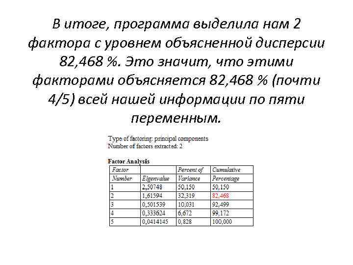 As a result, the program singled out 2 factors for us with a level of explained variance of 82.468%. This means that these factors account for 82.468% (nearly 4/5) of all our information on the five variables.
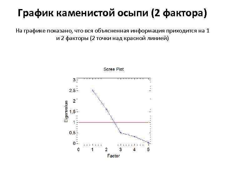 Scree plot (2 factors) The plot shows that all the explained information is due to factors 1 and 2 (2 dots above the red line)
 Factor loadings Press Tables (the second button on the left on the panel) Check the box next to Extraction Statistics → OK
 As you can see, the factor loadings at the level of tenths differ from those that we obtained by manual calculation and in Statistica. This is explained by the fact that in Statgraphics you cannot put your own correlation matrix and the program always considers it to be Pearson's coefficient, which is not adequate for data in order scales.
 Factor Plot Press Graphs (third button from the left of the panel) Check the box next to 2 D Factor Plot (if we had more than 2 factors, we would check the box next to 3 D Factor Plot to get a three-dimensional graph) → OK
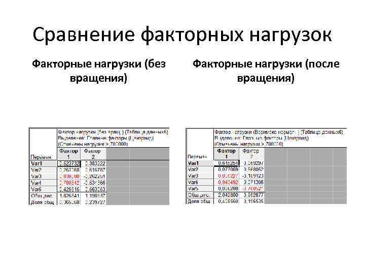
 We got the factor matrix after rotation. Segments (projections of points formed by factor loads) 2 and 5 are located close to the y-axis (tend to 0) and are removed from the x-axis. This means that the x-coordinates of these points (which corresponds to the first factor) are represented by low values (0, 6). Therefore scales 2 and 5 represent 1 factor. By the same principle, segment 1 indicates that scales 1, 3 and 4 represent the 2nd factor.
 Object Chart Click Graphs (third button from the left of the panel) Check the box next to 2 D Scatterplot (if we had more than 2 factors, we would check the box next to 3 D Scatterplot to get a 3D plot) → OK