Lecture
Topic No. 5 Tolerances and landings
Introduction
In the process of developing a product (machine, unit, unit), it is necessary to proceed from a given level of standardization and unification, which is determined by the coefficients of applicability, repeatability and inter-project unification. As the values of these coefficients increase, the economic efficiency of the product being developed during its production and operation increases. To increase the level of standardization and unification, it is necessary, already at the product design stage, to use a larger number of components produced by industry, and to strive for reasonable limitation of the development of original components. At the same time, the main issue in the development process is the accuracy of interchangeable parts, assemblies and components, primarily in terms of geometric parameters.
The interchangeability of parts, components and assemblies allows for aggregation as one of the standardization methods, to organize the supply of spare parts, to facilitate repairs, especially in difficult conditions, reducing it to a simple replacement of worn parts.
Interchangeability- the property of independently manufactured parts to take their place in an assembly unit without additional mechanical or manual processing during assembly, while ensuring the normal operation of the assembled products (assemblies, mechanisms).
From the very definition of interchangeability it follows that it is a prerequisite for the division of production, i.e. independent production of parts, components, assemblies, which are subsequently assembled sequentially into assembly units, and assembly units into a common system (mechanism, machine, device). Assembly can be carried out in two ways: with and without adjustment of assembled parts or assembly units. Assembly without adjustment is used in mass and mass production, and with adjustment - in single and small-scale production. When assembling without adjustment, parts must be manufactured with the required accuracy. However, interchangeability is not ensured by the accuracy of geometric parameters alone. It is necessary that the material, durability of parts, assembly units and components be consistent with the purpose and operating conditions of the final product. This interchangeability is called functional, and interchangeability in geometric parameters is a particular type of functional interchangeability.
Interchangeability can be complete or incomplete, external or internal.
Full interchangeability allows you to obtain specified quality indicators without additional operations during the assembly process.
At incomplete interchangeability During the assembly of assembly units and final products, operations related to the selection and adjustment of some parts and assembly units are allowed. It allows you to obtain specified technical and operational indicators of finished products with less precision of parts. At the same time, functional interchangeability should only be complete, and geometric interchangeability should be both complete and incomplete.
External interchangeability- this is the interchangeability of units and components in terms of operational parameters and connecting dimensions. For example, replacing an electric motor. Its operational parameters will be - power, rotation speed, voltage, current; Connecting dimensions include diameters, number and location of holes in the legs of the electric motor, etc.
Internal interchangeability is ensured by the accuracy of the parameters that are necessary for assembling parts into assemblies, and assemblies into mechanisms. For example, the interchangeability of ball bearings or rollers of rolling bearings, assemblies of the drive and driven shafts of the gearbox, etc.
The principles of interchangeability apply to parts, assembly units, components and final products.
Interchangeability is ensured by the accuracy of product parameters, in particular dimensions. However, during the manufacturing process, errors Х inevitably arise, the numerical values of which are found using the formula
where X is the specified value of the size (parameter);
Xi is the actual value of the same parameter.
Errors are divided into systematic, random and rough(misses).
The influence of random errors on measurement accuracy can be assessed using the methods of probability theory and mathematical statistics. Numerous experiments have proven that the distribution of random errors most often obeys the law of normal distribution, which is characterized by a Gaussian curve (Figure 1).

Figure 1 - Laws of distribution of random errors
a - normal; b – Maxwell; c – triangle (Simpson); r - equiprobable.
The maximum ordinate of the curve corresponds to the average value of a given size (with an unlimited number of measurements it is called the mathematical expectation and is denoted M(X).
Random errors or deviations from are plotted along the abscissa axis. The segments parallel to the ordinate axis express the probability of occurrence of random errors of the corresponding value. The Gaussian curve is symmetrical about the maximum ordinate. Therefore, deviations from the same absolute value, but different signs, are equally possible. The shape of the curve shows that small deviations (in absolute value) appear much more often than large ones, and the occurrence of very large deviations is almost unlikely. Therefore, permissible errors are limited to certain limiting values (V is the practical scattering field of random errors, equal to the difference between the largest and smallest measured dimensions in a batch of parts). The value is determined from the condition of sufficient accuracy at optimal costs for manufacturing products. With a regulated scattering field, no more than 2.7% of random errors can go beyond the limits. This means that out of 100 processed parts, no more than three may be defective. Further reduction in the percentage of defective products is not always advisable from a technical and economic point of view, because leads to an excessive increase in the practical stray field, and, consequently, an increase in tolerances and a decrease in the accuracy of products. The shape of the curve depends on the methods of processing and measuring products; exact methods give curve 1, which has a scattering field V1; using the high accuracy method corresponds to curve 2, for which V2
Depending on the adopted technological process, production volume and other circumstances, random errors can be distributed not according to Gauss’s law, but according to the equiprobability law (Fig. 1b), according to the triangle law (Fig. 1c), according to Maxwell’s law (Fig. 1d) and etc. The center of grouping of random errors can coincide with the average size coordinate (Fig. 1a) or shift relative to it (Fig. 1d).
It is impossible to completely eliminate the influence of the reasons causing processing and measurement errors; it is only possible to reduce the error by using more advanced technological processing processes. Size accuracy (of any parameter) is the degree of approximation of the actual size to the given size, i.e. The accuracy of the size is determined by the error. As the error decreases, the accuracy increases and vice versa.
In practice, interchangeability is ensured by limiting errors. As the errors decrease, the actual values of the parameters, in particular dimensions, approach the specified ones. With small errors, the actual dimensions differ so little from the specified ones that their error does not impair the performance of the products.
2. Tolerances and landings. The concept of quality
Basic terms and definitions are established by GOST 25346, GOST 25347, GOST 25348; tolerances and fits are established for sizes less than 1 mm, up to 500 mm, over 500 to 3150 mm.
Formulas (7) and (8) are derived from the following considerations. As follows from formulas (2) and (3), the largest and smallest limit sizes are equal to the sums of the nominal size and the corresponding maximum deviation:
![]() (9)
(9)
![]() (10)
(10)
Substituting into formula (5) the values of the maximum dimensions from the formula
Reducing similar terms, we obtain formula (7). Formula (8) is derived similarly.

Figure - Tolerance fields of the hole and shaft when landing with a gap (the hole deviations are positive, the shaft deviations are negative)
The tolerance is always a positive value, regardless of how it is calculated.
EXAMPLE. Calculate tolerance based on maximum dimensions and deviations. Given: = 20.010 mm; = 19.989 mm; = 10 µm; = -11 µm.
1). We calculate the tolerance through the maximum dimensions using formula (6):
Td = 20.010 - 19.989 = 0.021 mm
2). We calculate the tolerance for maximum deviations using formula (8):
Td = 10 - (-11) = 0.021 mm
EXAMPLE. Using the given symbols of the shaft and hole (shaft - , hole 20), determine the nominal and maximum dimensions, deviations and tolerances (in mm and microns).
2.2 Units of admission and the concept of qualifications
Dimensional accuracy is determined by tolerance - as the tolerance decreases, the accuracy increases, and vice versa.
Each technological method of processing parts is characterized by its economically justified optimal accuracy, but practice shows that with increasing dimensions, the technological difficulties of processing parts with small tolerances increase and the optimal tolerances under constant processing conditions increase somewhat. The relationship between economically achievable accuracy and dimensions is expressed by a conventional value called a tolerance unit.
Tolerance unit() expresses the dependence of the tolerance on the nominal size and serves as the basis for determining standard tolerances.
The tolerance unit, microns, is calculated using the formulas:
for sizes up to 500 mm
for sizes over 500 to 10000 mm
where is the average shaft diameter in mm.
In the above formulas, the first term takes into account the influence of processing errors, and the second - the influence of measurement errors and temperature errors.
Dimensions, even those with the same value, may have different accuracy requirements. It depends on the design, purpose and operating conditions of the part. Therefore, the concept is introduced quality .
Quality- a characteristic of the manufacturing accuracy of a part, determined by a set of tolerances corresponding to the same degree of accuracy for all nominal dimensions.
Tolerance (T) for qualifications, with some exceptions, is established according to the formula
where a is the number of tolerance units;
i(I) - tolerance unit.
According to the ISO system for sizes from 1 to 500 mm it is established 19 qualifications. Each of them is understood as a set of tolerances that ensure constant relative accuracy for a certain range of nominal sizes.
Tolerances of 19 qualifications are ranked in descending order of accuracy: 01, 0, 1, 2, 3,..17, and are conventionally designated IT01, IT0, IT1...IT17. here IT is the tolerance of holes and shafts, which means “ISO tolerance”.
Within one grade, “a” is constant, so all nominal sizes in each grade have the same degree of accuracy. However, tolerances in the same quality for different sizes still change, since with increasing sizes the tolerance unit increases, which follows from the above formulas. When moving from high-precision grades to coarse-precision grades, the tolerances increase due to an increase in the number of tolerance units, so the accuracy of the same nominal dimensions changes in different grades.
From all of the above it follows that:
The tolerance unit depends on the size and does not depend on the purpose, working conditions and methods of processing parts, that is, the tolerance unit allows you to evaluate the accuracy of various sizes and is a general measure of accuracy or the scale of tolerances of different qualifications;
Tolerances of the same dimensions in different qualifications are different, since they depend on the number of tolerance units “a”, that is, the qualifications determine the accuracy of the same nominal dimensions;
Various methods of processing parts have a certain economically achievable accuracy: “rough” turning allows you to process parts with rough tolerances; for processing with very small tolerances, fine grinding is used, etc., so the qualities actually determine the technology for processing parts.
Scope of qualifications:
Qualities from 01 to 4 are used in the manufacture of gauge blocks, gauges and counter gauges, parts of measuring instruments and other high-precision products;
Qualities from 5th to 12th are used in the manufacture of parts that primarily form interfaces with other parts of various types;
Qualities from 13 to 18 are used for parameters of parts that do not form mates and do not have a decisive influence on the performance of products. Maximum deviations are determined by GOST 25346-89.
Symbol for tolerance fields GOST 25347-82.
Symbol of maximum deviations and landings
Maximum deviations of linear dimensions are indicated in the drawings by conventional (letter) designations of tolerance fields or numerical values of maximum deviations, as well as letter designations of tolerance fields with simultaneous indication on the right in parentheses of numerical values of maximum deviations (Fig. 5.6, a... c). The fits and maximum deviations of the dimensions of the parts shown in assembled form in the drawing are indicated as a fraction: in the numerator - a letter designation or numerical value of the maximum deviation of the hole or a letter designation indicating its numerical value on the right in parentheses, in the denominator - a similar designation of the shaft tolerance field (Fig. 5.6, d, e). Sometimes, to indicate the fit, the maximum deviations of only one of the mating parts are indicated (Fig. 5.6, e).
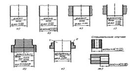
Rice. 5.6. Examples of designation of tolerance fields and fits in drawings
In the symbols of tolerance fields, it is necessary to indicate the numerical values of the maximum deviations in the following cases: for sizes not included in the series of normal linear dimensions, for example 41.5 H7 (+0.025); when assigning maximum deviations, the symbols of which are not provided for by GOST 25347-82, for example, for a plastic part (Fig. 5.6, g).
Maximum deviations should be assigned for all dimensions indicated on the working drawings, including non-matching and irrelevant dimensions. If maximum deviations for a size are not assigned, unnecessary costs are possible (when they try to get this size more accurate than necessary) or an increase in the weight of the part and excessive consumption of metal.
For a surface consisting of sections with the same nominal size, but different maximum deviations, the boundary between these sections is drawn with a thin solid line and the nominal size with the corresponding maximum deviations is indicated for each section separately.
The accuracy of smooth elements of metal parts, if deviations for them are not indicated directly after the nominal dimensions, but are specified in a general notation, are normalized either by qualifications (from 12 to 17 for sizes from 1 to 1000 mm), designated IT, or by accuracy classes (fine, medium, rough and very rough), established by GOST 25670-83. Tolerances for accuracy classes are designated t1, t2, t3 and t4 - respectively for accuracy classes - fine, medium, rough and very rough.
Unspecified maximum deviations for the dimensions of shafts and holes may be assigned both one-sided and symmetrical; for dimensions of elements other than holes and shafts, only symmetrical deviations are assigned. One-sided maximum deviations can be assigned both by qualifications (+IT or -IT) and by accuracy classes (± t/2), but it is also allowed by qualifications (± T/2). Quality 12 corresponds to the accuracy class “precise”, quality 14 - “medium”, quality 16 - “coarse”, quality 17 - “very rough”. Numerical values of unspecified maximum deviations are given in GOST 25670-83. For the dimensions of metal parts processed by cutting, it is preferable to assign unspecified maximum deviations according to quality 14 or “medium” accuracy class. Unspecified maximum deviations of nodes, radii of curvature and chamfers are assigned according to GOST 25670-83 depending on the quality or accuracy class of the unspecified maximum deviations of linear dimensions.
The connection of parts (assembly units) must ensure the accuracy of their position or movement, reliability of operation and ease of repair. In this regard, different requirements may be placed on the design of the connections. In some cases it is necessary to obtain a movable connection with a gap, in others - a fixed connection with interference.
Gap S is called the difference between the sizes of the hole and the shaft if the size of the hole is larger than the size of the shaft, i.e. S= D- d.
By interference N the difference between the sizes of the hole and the shaft is called if the size of the shaft is larger than the size of the hole. With a similar diameter ratio d And D the interference can be considered a negative clearance, i.e.
N= - S= - (D- d) = d- D , (12)
Clearances and interference are ensured not only by the dimensional accuracy of individual parts, but mainly by the ratio of the sizes of mating surfaces - the fit.
Landing call the nature of the connection of parts, determined by the size of the resulting gaps or interference.
Depending on the location of the tolerance fields, holes and shaft fits are divided into three groups:
Landings with clearance (provide clearance in the connection);
Preference fits (provide tension in the connection);
Transitional fits (make it possible to obtain both gaps and interference in connections).
Landings with a gap are characterized by maximum gaps - the largest and smallest. Largest clearance Smax is equal to the difference between the largest maximum hole size and the smallest maximum shaft size. Smallest clearance Smin equal to the difference between the smallest maximum hole size and the largest maximum shaft size. Landings with clearance also include fits in which the lower limit of the hole tolerance field coincides with the upper limit of the shaft tolerance field.
To create interference, the diameter of the shaft before assembly must be larger than the diameter of the hole. In the assembled state, the diameters of both parts in the mating zone are equalized. Maximum interference Nmax equal to the difference between the largest maximum shaft size and the smallest maximum hole size. Lowest interference Nmin equal to the difference between the smallest maximum shaft size and the largest maximum hole size.
Nmax=dmax-Dmin; Nmin= dmin-Dmax.
It is convenient to calculate the maximum interference, as well as the maximum clearances, using the maximum deviations:
![]()
![]() , (13)
, (13)
Transitional landings. The main feature of transitional fits is that in connections of parts belonging to the same batches, either gaps or interference can occur. Transitional fits are characterized by the largest gaps and the greatest interference.
Based on the calculations, we draw the following conclusions:
Since negative clearances are equal to positive interference and vice versa, to determine the values in the transition fit Smax And Nmax it is enough to calculate both maximum clearances or both maximum interference;
If calculated correctly Smin or Nmin will definitely turn out to be negative, and in absolute values they will be equal, respectively Nmax or Smax.
Fit tolerance TP equal to the sum of the hole and shaft tolerances. For clearance fits, the fit tolerance is equal to the clearance tolerance or the difference between the maximum clearances:
TP =T.S.= Smax- Smin , (14)
Similarly, it can be proven that for interference fits the fit tolerance is equal to the interference tolerance or interference difference:
TP =TN= Nmax- Nmin , (15)
3.1 Fit in the hole system and in the shaft system
A part in which the position of the tolerance field does not depend on the type of fit is called the main part of the system. The main part is a part whose tolerance field is basic for the formation of fits established in a given system of tolerances and fits.
Basics hole- a hole whose lower deviation is zero EI = 0. For the main hole, the upper deviation is always positive and equal to the tolerance ES = 0 = T; the tolerance field is located above the zero line and is directed towards increasing the nominal size.
Basic shaft- a shaft whose upper deviation is zero es = 0. For the main shaft Td = 0(ei) = the tolerance field is located below the zero line and is directed towards decreasing the nominal size.
Depending on which of the two mating parts is the main one, the tolerance and fit systems include two rows of fits: fits in the hole system - different gaps and tensions are obtained by connecting different shafts to the main hole; fits in the shaft system - various clearances and interferences are obtained by connecting various holes to the main shaft.
In the shaft system, the hole size limits for each fit are different, and three sets of special tools will be required for processing. Shaft system fits are used when connecting several parts with a smooth shaft (pin) using different fits. For example, in instrument making, precision axes of small diameter (less than 3 mm) are often made from smooth calibrated rods.
Achieving a variety of fits in a hole system requires significantly less specialized hole making tools. For this reason, this system is primarily used in mechanical engineering.
Additionally
Calibers for smooth cylindrical parts. Gauges are the main means of monitoring parts. They are used for manual inspection and are widely used in automatic parts inspection tools. The calibers provide high reliability of control.
According to their purpose, calibers are divided into two main groups: working calibers - pass-through R-PR and non-pass-through - R-NOT; control calibers - K-RP, K-NE and K-I.
Working gauges PR and NOT are intended to control products during their manufacturing process. These calibers are used by workers and quality control inspectors of the manufacturer.
Working gauges are called limit gauges, since their dimensions correspond to the maximum dimensions of the parts being controlled. Limit gauges allow you to determine whether the actual dimensions of parts are within tolerance. A part is considered suitable if it fits into the go-through gauge and does not fit into the non-go-through gauge.
The nominal dimensions of calibers are the dimensions that calibers would have to have if they were manufactured with perfect precision. Under this condition, the nominal size of the pass-through bracket will be equal to the largest maximum shaft size, and the nominal size of the no-go bracket will be equal to the smallest maximum shaft size. The nominal size of a go-through plug will be equal to the smallest limit size of the hole, and the nominal size of a no-go plug will be equal to the largest limit size of the hole.
The following requirements are imposed on control: control must be highly productive; time required for control, the time required to manufacture the part should be as short as possible; control must be reliable and economically feasible.
The economic feasibility of testing is determined by the cost of testing tools, the wear resistance of measuring surfaces, and the amount of narrowing of the tabulated tolerance field of the part.

For example, the greatest narrowing of the tolerance field is obtained in the case when the actual dimensions of the gauges coincide with their maximum dimensions located inside the tolerance field of the part.
The tabular tolerance narrowed due to calibers is called production tolerance. The tolerance expanded due to calibers is called guaranteed. The smaller the production capacity, the more expensive it is to manufacture parts, especially in more precise grades.
Limit calibers check the suitability of parts with tolerance from IT6 before IT 17, especially in mass and large-scale production.
In accordance with the Taylor principle, pass-through plugs and rings have full shapes and lengths equal to the mating lengths, and non-go-through gauges often have an incomplete shape: for example, staples are used instead of rings, as well as plugs that are incomplete in cross-sectional shape and shortened in the axial direction. Strict adherence to the Taylor principle is associated with certain practical inconveniences.
Control gauges TO-AND used for installing adjustable gauges and monitoring non-adjustable gauges, which are non-goable and are used for removal from service due to wear of the pass-through working brackets. Despite the small tolerance of control gauges, they still distort the established tolerance fields for the manufacture and wear of working gauges, therefore, whenever possible, control gauges should not be used. It is advisable, especially in small-scale production, to replace control gauges with gauge blocks or use universal measuring instruments.
GOST 24853-81 establishes the following manufacturing tolerances for smooth gauges: N- working gauges (plugs) for holes (Fig. 5.9, a) (Hs- the same calibers, but with spherical measuring surfaces); H\ - gauges (staples) for shafts (Fig. 5.9, b); HP- control gauges for staples.
For pass-through gauges that wear out during the inspection process, in addition to the manufacturing allowance, a wear allowance is provided. For sizes up to 500 mm, wear of PR calibers with a tolerance of up to IT 8 inclusive may go beyond the tolerance zone of parts by an amount at for traffic jams and y1 for staples; for PR calibers with tolerances from IT 9 to IT17 wear is limited to the pass limit, i.e. y = 0 And y1=0. It should be noted that the wear tolerance field reflects the average possible wear of the caliber.
Tolerance fields for all pass gauges N (N s) and H1 shifted inside the product tolerance zone by the amount z for plug gauges and z1 for clamp gauges.
With nominal sizes over 180 mm, the tolerance field of a non-goal gauge also shifts inside the tolerance field of the part by the amount a for plugs and a] for staples, creating a so-called safety zone introduced to compensate for the error of control by gauges of holes and shafts, respectively. Caliber tolerance range NOT for sizes up to 180 mm it is symmetrical and, accordingly, = 0 and l =0.
Shifting the tolerance fields of gauges and the wear limits of their passing sides inside the tolerance field of the part makes it possible to eliminate the possibility of distortion of the nature of fits and guarantee that the dimensions of suitable parts are obtained within the established tolerance fields.
Using the formulas of GOST 24853-81, the executive dimensions of the calibers are determined. Executive are the maximum caliber dimensions according to which a new caliber is manufactured. To determine these dimensions, the brackets are marked on the drawing with the smallest limit size with a positive deviation; for the plug and control gauge - their largest limit size with a negative deviation.
When marking, the caliber is marked with the nominal size of the part for which the caliber is intended, the letter designation of the tolerance field of the product, the numerical values of the maximum deviations of the product in millimeters (on working calibers), the type of caliber (for example, PR, NOT, K-AND) and the manufacturer's trademark.
Conclusion
In today's lesson we covered the following educational questions:
General information about interchangeability.
Tolerances and landings. The concept of quality.
Selecting a system of landings, tolerances and qualifications.
Self-study assignment
(1 hour for self-study)
Complete the lecture notes.
Get literature:
Main
Additional
1. Sergeev A.G., Latyshev M.V., Teregerya V.V. Standardization, metrology, certification. Tutorial. – M.: Logos, 2005. 560 pp. (pp. 355-383)
2. Lifits I.M. Standardization, metrology and certification. Textbook. 4th ed. –M.: Jurayt. 2004. 335 p.
3. Operation of chemical weapons and protective equipment. Tutorial. VAHZ, chipboard 1990. (inv. 2095).
4. Quality control of the development and production of weapons and military equipment. Edited by A.M. Smirnova. chipboard 2003. 274 p. (inv. 3447).
During the lesson, be prepared to:
1. Answer the teacher’s questions.
Present workbooks with practiced questions according to the assignment.
Literature
interchangeability part mechanical processing
1. Standardization, metrology, certification. Ed. Smirnova A.M. VU RKhBZ, dsp, 2001. 322 p. (inv. 3460).
2. Sergeev A.G., Latyshev M.V., Teregerya V.V. Standardization, metrology, certification. Tutorial. – M.: Logos, 2005. 560 p.
3. Metal technology. Textbook. Ed. V.A. Bobrovsky. -M. Voenizdat. 1979, 300 p.
Precision manufacturing of electronic equipment parts
Drawing and design documentation
While working on a course project, students complete an assembly drawing (or general view drawing) of the device body structure and working drawings of two parts.
The assembly drawing is drawn on a standard sheet of A3 paper , A4. First, the appropriate location of the projections of the device body structure, the necessary views and sections are determined, and then the scale of the drawing is selected. Due to the small size of semiconductor device packages, it is recommended to choose a scale of 5:1, 10:1. The assembly drawing shows overall and connecting dimensions, positions of assembly units, parts and standard products. Then a specification is drawn up for it.
Working drawings of parts are made on standard sheets of A4 paper (due to the small size of the parts). Recommended drawing scale is 10:1, 20:1. On the drawing of each part, all the necessary dimensions, maximum deviations for linear dimensions, for the shape and location of surfaces and for the roughness of the surfaces of the part are indicated. For more details on the accuracy of manufacturing parts and setting maximum deviations, see further in 6.4. The drawing indicates the material of the part, types of protective coatings, etc. When making assembly drawings and working drawings of parts, it is extremely important to be guided by ESKD GOST 2.104-68, GOST 2.108-68, GOST 2.109-73.
The settlement and explanatory note, drawn up on sheets of paper of 210´297 format in a thick cover, with a title page in the established form and bound, must include the following elements:
● assignment for a course project;
● description of the device;
● calculation of the strength of the device leads against inertial load;
● calculation of the strength of device leads under dynamic external influences;
● calculation of temperature stresses in the device body;
● conclusions;
● list of used literature;
The dimensions of a real product always have deviations from the actual (nominal) parameters. Today, permissible deviations in linear dimensions, shape and relative position of surfaces, as well as the surface roughness of the part are regulated by relevant standards. The parameters and their permissible deviations are indicated in technical documents according to the rules also specified in the standards. Compliance with the requirements of the standards when preparing technical documents is mandatory.
Permissible deviations in the dimensions of smooth elements of parts and the fit formed when connecting these elements. It is necessary that the actual dimensions of the product parts be maintained between two permissible limiting dimensional values, the difference of which forms a tolerance. For convenience, the nominal size is indicated, and each of the two maximum sizes is determined by its deviation from this nominal size. The absolute value and sign of the deviation are obtained by subtracting the nominal size from the corresponding maximum size (Fig. 6.9).
Rice. 6.9.
In the figure shown. In the example in 6.9, both shaft deviations have a negative sign (the tolerance field of the shaft is located below the zero line and at some distance from it), and both hole deviations have a positive sign (the tolerance field of the hole is located above the zero line and at some distance from it).
GOST 25347-82 provides for a certain position of the tolerance fields of holes and shafts relative to the zero line. In Fig. 6.10 shows such relative provisions and some tolerance fields for any size within the same interval of nominal sizes (over 6 to 10 mm) of the 6th and 9th qualifications. In this figure, solid lines show fields given in GOST 25347-82, dotted lines show fields not listed in GOST 25347-82 tables (they are not recommended for use), but calculated according to the rules of GOST 25347-82.
Actual size is the size established by measurement with permissible error.
Limit sizes - two maximum permissible sizes, between which the actual size must be or can be equal to.
Rice. 6.10
Nominal size is the size relative to which the maximum dimensions are determined and which also serves as the starting point for deviations. When designing products, nominal dimensions are obtained by calculation or chosen by the designer. As a rule, they must lie in the range of standard linear dimensions GOST 6636-69*.
The upper deviation is the algebraic difference between the largest limit and nominal sizes.
The lower deviation is the algebraic difference between the smallest limit and nominal sizes.
Tolerance ( 1T) – absolute value of the algebraic difference between the upper and lower deviations. For hole: IT=ES-EI; for shaft: IT=es-ei, Where ES And EI– upper and lower hole deviations; es And ei– upper and lower shaft deflections.
Tolerance field is a field limited by upper and lower deviations. It is determined by the tolerance value and the main deviation, indicating the position of the tolerance relative to the zero line. Standard tolerance fields for shafts and holes are indicated in the tables of GOST 25347-83.
The main deviation is the deviation closest to the zero line. Its value depends on the nominal size and location of the tolerance field and does not depend on the quality (Fig. 6.10).
Quality is a set of tolerances corresponding to the same degree of accuracy for all nominal sizes.
Shaft is a term used to designate the external (male) elements of parts.
Hole is a term used to designate internal (male) elements of parts.
The main shaft is a shaft whose upper deviation is zero (field n in Fig. 6.10).
The main hole is a hole whose lower deviation is zero (field H in Fig. 6.10).
The terms "shaft" and "hole" refer not only to cylindrical surfaces, but also to elements of parts of other shapes (for example, limited by two flat or curved surfaces).
Fit is the nature of the connection of parts, determined by the size of the resulting gaps or interferences, which are the difference between the sizes of the “hole” and the “shaft” before the connection. The fit determines the freedom of relative movement of the connected parts or the degree of resistance to their mutual movement, as well as the accuracy of the relative position of the connected parts. Taking into account the dependence of the location of the tolerance fields of the hole and shaft, fits are formed:
●with a gap (at which a gap is ensured in the connection - (the tolerance field of the hole is located above the tolerance field of the shaft), for example, as in Fig. 6.9);
●with interference (at which interference is ensured in the connection - the tolerance field of the hole is located under the tolerance field of the shaft);
●transitional (in which it is possible to obtain both a gap and an interference fit - the tolerance fields of the hole and shaft overlap partially or completely).
As a rule, fits are used in the hole system and in the shaft system.
●fits in a hole system – fits in which various gaps and tensions are formed by connecting various shafts to the main hole;
●fits and shaft system – fits in which various clearances and tensions are obtained by connecting various holes to the main shaft.
If elements of parts with tolerance fields of the main hole and the main shaft are connected to each other, the fit can be attributed to both one and the other system.
Because shaft systems require a greater number of specialized cutting and measuring tools to produce and inspect precise holes, in the vast majority of cases, bore system fits are used.
In this case, for all fits of a given nominal size, identical holes and different shafts are made, having certain permissible deviations for each fit.
Fittings in the shaft system usually have to be used in two cases:
1) when, with the same roller diameter, it is necessary to obtain different fits for several parts with the same nominal hole size;
2) when a part that has already been manufactured for fit in the shaft system is installed on the shaft or in the socket. At the same time, the shaft system must also accommodate all other parts installed on a roller of the same diameter.
In any connection, it is possible to obtain different clearances or interferences depending on the random actual dimensions of the shaft and hole within the tolerance. The higher the requirements for the accuracy of the connection and the certainty of the nature of the mating, the more accurately the parts included in it must be manufactured, i.e., the smaller the tolerances for the dimensions of the hole and shaft must be. Tolerances for sizes up to 500 mm are determined according to GOST 25346-82 as follows:
1. The entire range of sizes is divided into intervals (vmm) up to 3, over 3 to 6, over 6 to 10, etc.
2. The tolerance is set the same for any nominal size within the interval and depends on the accuracy (quality).
19 qualifications were accepted (01; 0;1; 2, ... 16, 17). To form different fits (connections with a certain nature of mating parts) in mechanical engineering and instrument making, qualifications from 5th to 12th are used. Qualities 14...17 are used to limit deviations of non-matching (free) dimensions, qualifications 01...4 are used for the manufacture of calibers.
GOST 25346-82 provides for 28 types of basic deviations (positions of the tolerance field relative to the zero line) for shafts and holes. The magnitude of the basic deviations depends on the nominal size and does not depend on the quality (tolerance value). The main deviations are indicated by letters of the Latin alphabet:
● for holes: A, B, C, CD, D, E, EF, FG, G, H, J, Js, K, M, N, P, R, S, T, U, V, X, Y, Z, ZA, ZB, ZC;
● for shafts: a, b, c, cd, d, e, ef, f, fg, g, h, j, js, k, m, n, p, r, s, t, u, v, x, y, z, za, zb, zc.
Some of these basic deviations with one nominal size for the 6th and 9th qualifications are shown in Fig. 6.10.
The main deviations are calculated according to the methodology set out by GOST 25346-82 g, according to two rules:
1) The general rule is that the main deviations of the hole and shaft, indicated by the same letter, must be symmetrical relative to the zero line, for example G And g(Fig. 6.10);
2) Special rule - two corresponding fits in the hole system and in the shaft system, in which a hole of a given quality is connected to the shaft of the next more accurate quality (for example, H7/n6 and N7/h6), must have the same clearances and interference. The rule is valid for size intervals greater than 3 mm.
On any working drawing, all dimensions to be made according to this document must have instructions on permissible deviations.
Maximum dimensional deviations are indicated in one of three ways (GOST 2.307-68):
1) in conventionally designated tolerance fields according to GOST 25347-82 (for example, 8 N 7; 5f 8; 12Js 7);
2) numerical values of maximum deviations in millimeters. In case of asymmetrical deviations, they are indicated as follows: upper – at the top, lower – at the bottom, immediately after the nominal size in a font smaller than the main one (for example, 5 +0.03 ; ).
If the deviation is symmetrical, it is indicated in the main font (for example, 8 ± 0.007). Deviation designations must end with a significant figure, except in cases where the upper and lower deviations have a different number of decimal places (for example, );
3) combining the first and second methods, with the numerical values of deviations written in parentheses after the symbols (for example, 8 N 7 (+0.015) ; 5f ; 12Js 7 (±0.009)).
If necessary, the assembly drawings indicate which fit should be made in a particular interface. In this case, the nominal mating size is indicated, the same for both mating elements (hole and shaft), and immediately after it there are designations of the tolerance fields for each element starting from the hole, for example:
Or 8 N 7-g 6 or 8 N 7/g 6 .
●on the drawings of parts 18 N 8; 18f 7;
●on assembly drawings 18 N 8/f 7.
Additionally, numerical values of permissible deviations should be given in the following cases:
● if the nominal size does not fall within the range of preferred numbers GOST 6636-69* (for example, 39 N 7 (+0.025));
● for all basic hole deviations, except N(for example, when planting holes that are not in the system).
On the working drawing of the part, the dimensions of chamfers, rounding and bending radii can be indicated without permissible deviations; width and depth of grooves for tool exit; zones of different roughness of the same surface; zones of heat treatment, coating, finishing, corrugation, notching, diameters of corrugated and notched surfaces, as well as reference dimensions (for example, the size of the workpiece, if it does not change according to this drawing).
It is worth saying that for several dimensions of the same relatively low accuracy, permissible deviations are not set next to each of them, but a general inscription is given on the drawing field (see below).
Assembly drawings should indicate the nominal values and permissible deviations of the dimensions made according to this document (for example, dimensions determining the relative position of welded parts, or dimensions obtained by adjustment), as well as all connecting dimensions.
Overall dimensions on assembly drawings are given without maximum deviations.
Maximum dimensional deviations with unspecified tolerances are established by the GOST 25670-83 standard, which applies to smooth elements of metal parts processed by cutting, and is recommended for metal parts processed by other methods, if the permissible deviations are specified in a general entry.
Unspecified maximum deviations of linear dimensions, except for radii of curvatures and chamfers, can be assigned either according to the qualifications of GOST 25346-82, or according to the accuracy classes of GOST 25670-83. The numerical values of maximum deviations by accuracy classes are established by rough rounding of the numerical values of deviations by qualification. In table 6.17 shows the approximate correspondence between accuracy classes and qualifications.
Unspecified maximum deviations of the radii of roundings, chamfers and angles are established depending on the quality or accuracy class of the unspecified maximum deviations of linear dimensions.
Table 6.17
Table 6.18
| Linear dimensions, radii of rounding and chamfers | Angles | ||||||
| Size range, mm | Maximum deviations, mm | Interval of lengths of the smaller side of the angle | Limit deviations | ||||
| linear dimensions | radii of curves and chamfers | ang. units | mm per 100 mm length | ||||
| ± | Minus t 2 | +t 2 | |||||
| From 0.3 to 0.5 | - | - | - | ±0.1 | To 10 | ±1 0 | 1.8± |
| Over 0.5 to 1 | ±0.1 | Minus 0.2 | +0.2 | ||||
| Over 1 to 3 | ±0.2 | ||||||
| Over 3 to 6 | ±0.1 | Minus 0.2 | +0.2 | ±0.3 | |||
| Over 6 to 10 | ±0.2 | Minus 0.4 | +0.4 | ±0.5 | Over 10 to 40 | ±30" | ±0.9 |
| Over 10 to 18 | |||||||
| Over 18 to 30 | |||||||
| Over 30 to 50 | ±0.3 | Minus 0.6 | +0.6 | ±1 | Over 40 to 160 | ±20’ | ±0.6 |
| Over 50 to 80 | |||||||
| Over 80 to 120 | |||||||
| Over 120 to 180 | ±0.5 | Minus | +1 | ±2 | Over 160 to 500 | ±10’ | ±0.3 |
| Over 180 to 250 | |||||||
| Over 250 to 350 | |||||||
| Over 350 to 400 | ±0.8 | Minus 1.6 | +1.6 | ±1 | |||
| Over 400 to 500 |
In table 6.18 shows the values of maximum dimensional deviations according to the “medium” accuracy class of GOST 25670-83.
An example of a recommended general inscription in drawings of educational projects: unspecified maximum deviations of dimensions - according to H 14, n 14, ± t 2 /2. It should be borne in mind that such a solution is most justified for the linear dimensions of elements obtained by cutting. For the majority of free dimensions obtained by casting, stamping, and pressing, it may be more acceptable to have a symmetrical arrangement of the tolerance field for all dimensions.
After the nominal size in the drawings, symbols + t, minus t, and ± t/2 is not used. If a general inscription for large permissible deviations is not made, then after the nominal size the tolerance field for quality should be indicated (for example, 5 N 14). For dimensions that do not relate to shafts or holes, in this case only the numerical value of the tolerance field of quality or accuracy class with a symmetrical arrangement is set (for example, 8±0.18 or 8±0.2).
Tolerances of shape and location of surfaces. Basic terms and definitions are given in GOST 24642-81. Let's introduce some of them.
Shape deviation is the greatest distance from the points of the real surface (profile) to the adjacent surface (profile) along the normal to the adjacent surface (profile).
Shape tolerance is the largest permissible shape deviation value.
The common axis is a straight line relative to which the greatest deviation of the axes of several considered surfaces of revolution within the limits of the length of these surfaces has a minimum value.
Deviation from parallelism of planes is the difference ∆ of the largest and smallest distances between planes within the normalized area.
Deviation from the plane is the greatest distance ∆ from the points of the real surface to the adjacent plane within the normalized area.
Radial runout is the difference between the largest and smallest distances from the points of the real profile of the surface of revolution to the base axis in a section by a plane perpendicular to the base axis.
End runout is the difference ∆ of the largest and smallest distances from the points of the real profile of the end surface to the plane perpendicular to the base axis.
Positional deviation is the greatest distance ∆ between the actual location of an element (its center, axis or plane of symmetry) and its nominal location within the normalized area.
Positional tolerance:
1) tolerance in the diametrical position - twice the maximum permissible value of the positional deviation of the element;
2) tolerance in radius terms - the largest permissible value of the positional deviation of the element.
Dependent tolerance for the location of smooth holes - for fasteners - the minimum tolerance value, which is allowed to be exceeded during the manufacture of products by an amount corresponding to the deviation of the actual size of the element downward from the largest limiting size of the rod and upward from the smallest limiting hole size.
Tolerances for the shape and location of the surface are assigned, as a rule, only if these deviations must be less than the tolerance for the linear dimension. When shape and position tolerances are not specified, it is assumed that deviations may lie within the linear dimension tolerance.
Methods for symbolizing tolerances of the shape and location of surfaces are taken into account by the standards ST SEV 368-76 and GOST 2.308-79.
Signs of some types of tolerance:
straightness -
Flatness
roundness O
cylindricity /○/
parallelism //
Positional
perpendicularity ┴
X-axis intersections
Alignment
Face runout,
Radial runout
symmetry ÷
The sign and numerical value of the tolerance, as well as the designation of the base from which the measurement is made, are inscribed in a frame made by solid thin lines or lines of the same thickness with the numbers. The frame is divided into two or three fields. In the first of them, the tolerance sign is given, in the second - the tolerance value in millimeters, in the third (if extremely important) - the letter designation of the base (bases), if the frame is not connected to a blackened triangle adjacent to the base.
In Fig. 6.11 shows the simplest cases of designating tolerances. The sign α indicates that the tolerance is dependent. The height of the signs within the frames and equilateral blackened triangles is equal to the height of the dimensional numbers. The width of the frame is twice the height of the pin.
When making holes for fasteners, the distance between the axes of real holes in the parts being connected, like any other linear dimension, cannot be made equal to the nominal size. When assembling parts, these holes are not completely aligned. If the deviation of the interaxial distance from the nominal value is minimal, then the closest coincidence of the connected holes is obtained and the rod of the fastener (screw, stud, rivet, etc.) is placed in the resulting gap with the required gap.
GOST 14140-81 sets out the method for determining positional tolerance T in diametrical terms, i.e. twice the maximum permissible distance between the actual location of the hole axis and its nominal location. It contains tables from which, based on the value of this tolerance, you can set the permissible deviations of the dimensions coordinating the axes of the holes.
Rice. 6.11
Surface roughness. Any surface of a solid body, no matter how carefully and no matter how it is made, has micro-irregularities. These irregularities should not be mixed with macro-irregularities that create waviness and distortion of the shape of surfaces (for example, deviation from flatness, cylindricity, etc.).
When magnified by tens and hundreds of times, the profile of the section (for example, normal to the nominal surface specified in the technical documentation) is presented in a form similar to that shown in Fig. 6.12.
Base length L used to highlight irregularities that characterize surface roughness. Within the base length L the standard deviation of the profile to the center line is minimal; y– profile deviation; y p– profile protrusion height, at V– depth of the profile depression.
The surface roughness is judged by the size and shape of micro-irregularities in the normal section (GOST 25142-82).
Measurements are taken at the base length L, selected according to a certain method. GOST 2789-73* establishes several roughness parameters, of which the most often used Rz And R a.
Height of profile irregularities at ten points Rz– the average absolute value of the sums of the heights of the five largest protrusions of the profile and the depths of the five largest depressions of the profile within the base length (see Fig. 6.12):
Arithmetic mean deviation of the profile R a– arithmetic mean of the absolute values of profile deviations within the base length:
R a= , or approximately, R a = .
In educational projects, if there are no special requirements for them, it is recommended to limit oneself to indicating only one of these two surface roughness parameters and only their maximum values for each of the 14 roughness classes according to GOST 2789-73 *, see table. 6.11 (Symbol R a omitted in notation).
Roughness is assigned depending on the requirements for the connection or the appearance of the parts, or on the selected technological process for surface formation. Roughness must be indicated for all surfaces made according to this drawing. In the designation of surface roughness, three types of signs are used:
√ – when the method of obtaining the surface is not specified (preferred sign);
√ – when formed by removing a layer of material;
√ – when the surface is obtained without removing a layer of material or when this surface is not formed according to a given drawing.
The dimensions of the sign are indicated as follows:
Where h– the height of the dimensional numbers in the drawing, N = 1.5 h. The sign is placed with its tip on the designated surface from the outside onto the material or (also) on an extension line from this surface. The parameter and its value are indicated in accordance with Fig. 6.13, a, b.
Table 6.19
| Roughness class | Maximum parameter value according to GOST 2789-73 * |
| Rz 320 | |
| Rz 160 | |
| Rz 80 | |
| Rz 40 | |
| Rz 20 | |
| 2.5 | |
| 1.25 | |
| 0.63 | |
| 0.32 | |
| 0.16 | |
| 0.08 | |
| 0.04 | |
| Rz 0.1 | |
| Rz 0.05 |
If a large number of surfaces have the same roughness, then in the upper right corner of the drawing a designation similar to that shown in Fig. 6.13, d. This means that surfaces for which the roughness is not indicated on the drawing should have it no rougher Rz 40.
For small holes, the roughness is marked on the measuring line (see also Fig. 6.13).
The designation of roughness is specified in detail in GOST 2.309-85.
a B C
Rice. 6.13
Recommendations for choosing fits, tolerance ranges and surface roughness. High quality and reliable operation of the entire product and each of its parts are largely ensured by the correct choice of manufacturing tolerances and surface roughness of parts.
To obtain a particular quality of surfaces, providing, for example, the necessary properties of mating parts, various technological processes are used. In table 6.20 shows the possibilities of shaping processes of both non-mating and mating surfaces of metal parts. When mating two parts, use basic deviations from A(A) before G(g) makes it possible to land with a gap from J(j) before N(n) – transitional from P(p) before Z(x) with interference. In order to reduce the labor intensity and cost of products, enterprises limit the number of plantings used. When manufacturing metal parts of radio-electronic equipment for fixed connections, interference fits of the type N 7/r6, N 8/s7, for parts made of fiberglass – N 8/u 8. It is worth saying that for fixed connections of plastic parts it is recommended to use only transitional fits like N 8/To 8, N 9/To 9, N 10/To 10. It is not recommended to use landings rougher than 11th quality.
Table 6.20
| Technological process | Accuracy of linear dimensions, quality | Roughness | ||||
| regular | increased | |||||
| Casting | In sandy forms | Rz 160 | ||||
| By investment models | Rz 20 | |||||
| In the chill mold | Rz 40 | |||||
| Under pressure | Rz 20 | |||||
| Cold stamping | Felling | Diameters | Rz 40 | |||
| Lengths | ||||||
| Ledges | ||||||
| With stripping | 2,5 | |||||
| Bending | ± t 3 */2 | ± t 2 */2 | ||||
| Turning | 12…14 | Rz 20…0,63 | ||||
| Milling | 12…14 | Rz 40…0,63 | ||||
| Machining | Grinding | 2,5…0,16 | ||||
| Drilling | Rz 40 | |||||
| Deployment | 0,63 | |||||
| Boring holes | ||||||
| Tolerance of shape and location, mm | ||||||
| Flat base surfaces | 0.05…0.03 // 0.1…0.02 ┴ 0.1…0.05 per 100 mm | 2,5 | ||||
* Indicate the numerical value on the drawing.
All mating metal surfaces must have a roughness of no rougher than grade 6 ( R a 2.5); unmatched in packages of microcircuits and other semiconductor products usually have class 5 ( Rx 20). At the point of contact with glass, the metal surface must have a cleanliness class of 5–7 ( Rz 20 … - R a 1.25).
The roughness of glass is, as a rule, 25 microns (5th class and more precisely), the roughness of plastic parts is 6–9th classes. Ceramic and metal-ceramic parts after sintering have dimensions with tolerances of 10 - 12 grades and surface roughness R a 2,5.
In the manufacture of semiconductor devices and microcircuits, high demands are placed on the cleanliness of the surfaces of contact pads for connecting leads (it must be at least 8–9 classes ( R a 0.63...0.32) and especially high - to the cleanliness of the surface of the substrate, which after polishing must correspond to class 14 ( Rz 0.05).
In cases of extreme production importance, the drawings stipulate tolerances for the shape and location of the surface, which form part of the size tolerance: in connections of normal accuracy » 60%; in high-precision connections » 40%; in high precision connections » 25%. For cylindrical surfaces, the shape tolerance limits the radius deviations and therefore amounts to 30, 20 and 12% of the size tolerance, respectively.
To main
section four
Tolerances and landings.
Measuring tool
Chapter IX
Tolerances and landings
1. The concept of interchangeability of parts
In modern factories, machine tools, cars, tractors and other machines are produced not in units or even in tens or hundreds, but in thousands. With such a production scale, it is very important that each part of the machine fits exactly into its place during assembly without any additional fitting. It is equally important that any part entering the assembly allows its replacement by another of the same purpose without any damage to the operation of the entire finished machine. Parts that satisfy such conditions are called interchangeable.
Interchangeability of parts- this is the property of parts to take their places in units and products without any preliminary selection or adjustment in place and perform their functions in accordance with the prescribed technical conditions.
2. Mating parts
Two parts that are movably or stationarily connected to each other are called mating. The size by which these parts are connected is called mating size. Dimensions for which parts are not connected are called free sizes. An example of mating dimensions is the diameter of the shaft and the corresponding diameter of the hole in the pulley; An example of free dimensions is the outer diameter of a pulley.
To obtain interchangeability, the mating dimensions of the parts must be accurately executed. However, such processing is complex and not always practical. Therefore, technology has found a way to obtain interchangeable parts while working with approximate accuracy. This method consists in the fact that for various operating conditions of a part, permissible deviations in its dimensions are established, under which flawless operation of the part in the machine is still possible. These deviations, calculated for various operating conditions of the part, are built in a specific system called admission system.
3. Concept of tolerances
Size specifications. The calculated size of the part, indicated on the drawing, from which deviations are measured, is called nominal size. Typically, nominal dimensions are expressed in whole millimeters.
The size of the part actually obtained during processing is called actual size.
The dimensions between which the actual size of a part can fluctuate are called extreme. Of these, the larger size is called largest size limit, and the smaller one - smallest size limit.
Deviation is the difference between the maximum and nominal dimensions of a part. In the drawing, deviations are usually indicated by numerical values at a nominal size, with the upper deviation indicated above and the lower deviation below.
For example, in size, the nominal size is 30, and the deviations will be +0.15 and -0.1.
The difference between the largest limit and nominal sizes is called upper deviation, and the difference between the smallest limit and nominal sizes is lower deviation. For example, the shaft size is . In this case, the largest limit size will be:
30 +0.15 = 30.15 mm;
the upper deviation will be
30.15 - 30.0 = 0.15 mm;
the smallest size limit will be:
30+0.1 = 30.1 mm;
the lower deviation will be
30.1 - 30.0 = 0.1 mm.
Manufacturing approval. The difference between the largest and smallest limit sizes is called admission. For example, for a shaft size, the tolerance will be equal to the difference in the maximum dimensions, i.e.
30.15 - 29.9 = 0.25 mm.
4. Clearances and interference
If a part with a hole is mounted on a shaft with a diameter , i.e., with a diameter under all conditions less than the diameter of the hole, then a gap will necessarily appear in the connection of the shaft with the hole, as shown in Fig. 70. In this case, landing is called mobile, since the shaft can rotate freely in the hole. If the size of the shaft is, that is, always larger than the size of the hole (Fig. 71), then when connecting the shaft will need to be pressed into the hole and then the connection will turn out preload


Based on the above, we can draw the following conclusion:
the gap is the difference between the actual dimensions of the hole and the shaft when the hole is larger than the shaft;
interference is the difference between the actual dimensions of the shaft and the hole when the shaft is larger than the hole.
5. Fit and accuracy classes
Landings. Plantings are divided into mobile and stationary. Below we present the most commonly used plantings, with their abbreviations given in parentheses.

Accuracy classes. It is known from practice that, for example, parts of agricultural and road machines can be manufactured less accurately than parts of lathes, cars, and measuring instruments without harming their operation. In this regard, in mechanical engineering, parts of different machines are manufactured according to ten different accuracy classes. Five of them are more accurate: 1st, 2nd, 2a, 3rd, Za; two are less accurate: 4th and 5th; the other three are rough: 7th, 8th and 9th.
To know what accuracy class the part needs to be manufactured in, on the drawings next to the letter indicating the fit, a number indicating the accuracy class is placed. For example, C 4 means: sliding landing of the 4th accuracy class; X 3 - running landing of the 3rd accuracy class; P - tight fit of 2nd accuracy class. For all 2nd class landings, the number 2 is not used, since this accuracy class is used especially widely.
6. Hole system and shaft system
There are two systems for arranging tolerances - the hole system and the shaft system.
The hole system (Fig. 72) is characterized by the fact that for all fits of the same degree of accuracy (same class), assigned to the same nominal diameter, the hole has constant maximum deviations, while a variety of fits is obtained by changing the maximum shaft deviations.

The shaft system (Fig. 73) is characterized by the fact that for all fits of the same degree of accuracy (same class), referred to the same nominal diameter, the shaft has constant maximum deviations, while the variety of fits in this system is carried out within by changing the maximum deviations of the hole.
In the drawings, the hole system is designated by the letter A, and the shaft system by the letter B. If the hole is made according to the hole system, then the nominal size is marked with the letter A with a number corresponding to the accuracy class. For example, 30A 3 means that the hole must be processed according to the hole system of the 3rd accuracy class, and 30A - according to the hole system of the 2nd accuracy class. If the hole is machined using the shaft system, then the nominal size is marked with a fit and the corresponding accuracy class. For example, a hole 30С 4 means that the hole must be processed with maximum deviations according to the shaft system, according to a sliding fit of the 4th accuracy class. In the case when the shaft is manufactured according to the shaft system, the letter B and the corresponding accuracy class are indicated. For example, 30B 3 will mean processing a shaft using a 3rd accuracy class shaft system, and 30B - using a 2nd accuracy class shaft system.
In mechanical engineering, the hole system is used more often than the shaft system, since it is associated with lower costs for tools and equipment. For example, to process a hole of a given nominal diameter with a hole system for all fits of one class, only one reamer is required and to measure a hole - one / limit plug, and with a shaft system, for each fit within one class a separate reamer and a separate limit plug are needed.
7. Deviation tables
To determine and assign accuracy classes, fits and tolerance values, special reference tables are used. Since permissible deviations are usually very small values, in order not to write extra zeros, in tolerance tables they are indicated in thousandths of a millimeter, called microns; one micron is equal to 0.001 mm.
As an example, a table of the 2nd accuracy class for a hole system is given (Table 7).
The first column of the table gives the nominal diameters, the second column shows the hole deviations in microns. The remaining columns show various fits with their corresponding deviations. The plus sign indicates that the deviation is added to the nominal size, and the minus sign indicates that the deviation is subtracted from the nominal size.
As an example, we will determine the fit movement in a hole system of the 2nd accuracy class for connecting a shaft with a hole with a nominal diameter of 70 mm.
The nominal diameter 70 lies between the sizes 50-80 placed in the first column of the table. 7. In the second column we find the corresponding hole deviations. Therefore, the largest limit hole size will be 70.030 mm, and the smallest 70 mm, since the lower deviation is zero.
In the column “Motion fit” against the size from 50 to 80, the deviation for the shaft is indicated. Therefore, the largest maximum shaft size is 70-0.012 = 69.988 mm, and the smallest maximum size is 70-0.032 = 69.968 mm.
Table 7
Limit deviations of the hole and shaft for the hole system according to the 2nd accuracy class
(according to OST 1012). Dimensions in microns (1 micron = 0.001 mm)


Control questions 1. What is called the interchangeability of parts in mechanical engineering?
2. Why are permissible deviations in the dimensions of parts assigned?
3. What are nominal, maximum and actual sizes?
4. Can the maximum size be equal to the nominal size?
5. What is called tolerance and how to determine tolerance?
6. What are the upper and lower deviations called?
7. What is clearance and interference called? Why are clearance and interference provided in the connection of two parts?
8. What types of landings are there and how are they indicated on the drawings?
9. List the accuracy classes.
10. How many landings does the 2nd accuracy class have?
11. What is the difference between a bore system and a shaft system?
12. Will the hole tolerances change for different fits in the hole system?
13. Will the maximum shaft deviations change for different fits in the hole system?
14. Why is the hole system used more often in mechanical engineering than the shaft system?
15. How are symbols for deviations in hole dimensions placed on the drawings if the parts are made in a hole system?
16. In what units are the deviations indicated in the tables?
17. Determine using the table. 7, deviations and tolerance for the manufacture of a shaft with a nominal diameter of 50 mm; 75 mm; 90 mm.
Chapter X
Measuring tool
To measure and check the dimensions of parts, a turner has to use various measuring tools. For not very accurate measurements, they use measuring rulers, calipers and bore gauges, and for more accurate ones - calipers, micrometers, gauges, etc.
1. Measuring ruler. Calipers. Bore gauge
Yardstick(Fig. 74) is used to measure the length of parts and ledges on them. The most common steel rulers are from 150 to 300 mm long with millimeter divisions.

The length is measured by directly applying a ruler to the workpiece. The beginning of the divisions or the zero stroke is combined with one of the ends of the part being measured and then the stroke on which the second end of the part falls is counted.
Possible measurement accuracy using a ruler is 0.25-0.5 mm.

Calipers (Fig. 75, a) are the simplest tool for rough measurements of the external dimensions of workpieces. A caliper consists of two curved legs that sit on the same axis and can rotate around it. Having spread the legs of the calipers slightly larger than the size being measured, lightly tapping them on the part being measured or some hard object moves them so that they come into close contact with the outer surfaces of the part being measured. The method of transferring the size from the part being measured to the measuring ruler is shown in Fig. 76.

In Fig. 75, 6 shows a spring caliper. It is adjusted to size using a screw and nut with a fine thread.
A spring caliper is somewhat more convenient than a simple caliper, as it maintains the set size.
Bore gauge. For rough measurements of internal dimensions, use the bore gauge shown in Fig. 77, a, as well as a spring bore gauge (Fig. 77, b). The device of the bore gauge is similar to that of a caliper; Measurement with these instruments is also similar. Instead of a bore gauge, you can use calipers by moving its legs one after the other, as shown in Fig. 77, v.

The measurement accuracy with calipers and bore gauges can be increased to 0.25 mm.
2. Vernier caliper with reading accuracy 0.1 mm
The accuracy of measurement with a measuring ruler, calipers, or bore gauge, as already indicated, does not exceed 0.25 mm. A more accurate tool is a caliper (Fig. 78), which can be used to measure both the external and internal dimensions of the workpieces. When working on a lathe, calipers are also used to measure the depth of a recess or shoulder.

The caliper consists of a steel rod (ruler) 5 with divisions and jaws 1, 2, 3 and 8. Jaws 1 and 2 are integral with the ruler, and jaws 8 and 3 are integral with frame 7, sliding along the ruler. Using screw 4, you can secure the frame to the ruler in any position.

To measure the outer surfaces use jaws 1 and 8, to measure the internal surfaces use jaws 2 and 3, and to measure the depth of the recess use rod 6 connected to frame 7.
On frame 7 there is a scale with strokes for reading fractional fractions of a millimeter, called vernier. The vernier allows measurements to be made with an accuracy of 0.1 mm (decimal vernier), and in more accurate calipers - with an accuracy of 0.05 and 0.02 mm.
Vernier device. Let's consider how a vernier reading is made on a vernier caliper with an accuracy of 0.1 mm. The vernier scale (Fig. 79) is divided into ten equal parts and occupies a length equal to nine divisions of the ruler scale, or 9 mm. Therefore, one division of the vernier is 0.9 mm, i.e. it is shorter than each division of the ruler by 0.1 mm.
If you close the jaws of the caliper closely, the zero stroke of the vernier will exactly coincide with the zero stroke of the ruler. The remaining vernier strokes, except the last one, will not have such a coincidence: the first vernier stroke will not reach the first stroke of the ruler by 0.1 mm; the second stroke of the vernier will not reach the second stroke of the ruler by 0.2 mm; the third stroke of the vernier will not reach the third stroke of the ruler by 0.3 mm, etc. The tenth stroke of the vernier will exactly coincide with the ninth stroke of the ruler.
If you move the frame so that the first stroke of the vernier (not counting the zero) coincides with the first stroke of the ruler, then between the jaws of the caliper you will get a gap of 0.1 mm. If the second stroke of the vernier coincides with the second stroke of the ruler, the gap between the jaws will already be 0.2 mm, if the third stroke of the vernier coincides with the third stroke of the ruler, the gap will be 0.3 mm, etc. Consequently, the vernier stroke that exactly coincides with which - using a ruler stroke, shows the number of tenths of a millimeter.
When measuring with a caliper, they first count a whole number of millimeters, which is judged by the position occupied by the zero stroke of the vernier, and then look at which vernier stroke coincides with the stroke of the measuring ruler, and determine tenths of a millimeter.
In Fig. 79, b shows the position of the vernier when measuring a part with a diameter of 6.5 mm. Indeed, the zero line of the vernier is between the sixth and seventh lines of the measuring ruler, and, therefore, the diameter of the part is 6 mm plus the reading of the vernier. Next, we see that the fifth stroke of the vernier coincides with one of the strokes of the ruler, which corresponds to 0.5 mm, so the diameter of the part will be 6 + 0.5 = 6.5 mm.
3. Vernier depth gauge
To measure the depth of recesses and grooves, as well as to determine the correct position of the ledges along the length of the roller, use a special tool called depth gauge(Fig. 80). The design of the depth gauge is similar to that of a caliper. Ruler 1 moves freely in frame 2 and is fixed in it in the desired position using screw 4. Ruler 1 has a millimeter scale, on which, using vernier 3, located on frame 2, the depth of the recess or groove is determined, as shown in Fig. 80. The reading on the vernier is carried out in the same way as when measuring with a caliper.

4. Precision caliper
For work performed with greater accuracy than those considered so far, use precision(i.e. accurate) calipers.
In Fig. 81 shows a precision caliper from the plant named after. Voskov, having a measuring ruler 300 mm long and a vernier.

The length of the vernier scale (Fig. 82, a) is equal to 49 divisions of the measuring ruler, which is 49 mm. This 49 mm is precisely divided into 50 parts, each equal to 0.98 mm. Since one division of the measuring ruler is equal to 1 mm, and one division of the vernier is equal to 0.98 mm, we can say that each division of the vernier is shorter than each division of the measuring ruler by 1.00-0.98 = 0.02 mm. This value of 0.02 mm indicates that accuracy, which can be provided by the vernier of the considered precision caliper when measuring parts.


When measuring with a precision caliper, to the number of whole millimeters passed by the zero stroke of the vernier, one must add as many hundredths of a millimeter as the vernier stroke that coincides with the stroke of the measuring ruler shows. For example (see Fig. 82, b), along the ruler of the caliper, the zero stroke of the vernier passed 12 mm, and its 12th stroke coincided with one of the strokes of the measuring ruler. Since matching the 12th line of the vernier means 0.02 x 12 = 0.24 mm, the measured size is 12.0 + 0.24 = 12.24 mm.
In Fig. 83 shows a precision caliper from the Kalibr plant with a reading accuracy of 0.05 mm.
The length of the vernier scale of this caliper, equal to 39 mm, is divided into 20 equal parts, each of which is taken as five. Therefore, against the fifth stroke of the vernier there is the number 25, against the tenth - 50, etc. The length of each division of the vernier is ![]()
From Fig. 83 it can be seen that with the jaws of the caliper closed tightly, only the zero and last strokes of the vernier coincide with the strokes of the ruler; the rest of the vernier strokes will not have such a coincidence.
If you move frame 3 until the first stroke of the vernier coincides with the second stroke of the ruler, then between the measuring surfaces of the caliper jaws you will get a gap equal to 2-1.95 = 0.05 mm. If the second stroke of the vernier coincides with the fourth stroke of the ruler, the gap between the measuring surfaces of the jaws will be equal to 4-2 X 1.95 = 4 - 3.9 = 0.1 mm. If the third stroke of the vernier coincides with the next stroke of the ruler, the gap will be 0.15 mm.
The counting on this caliper is similar to that described above.
A precision caliper (Fig. 81 and 83) consists of ruler 1 with jaws 6 and 7. Markings are marked on the ruler. Frame 3 with jaws 5 and 8 can be moved along ruler 1. A vernier 4 is screwed to the frame. For rough measurements, frame 3 is moved along ruler 1 and, after securing with screw 9, a count is taken. For accurate measurements, use the micrometric feed of the frame 3, consisting of a screw and nut 2 and a clamp 10. Having clamped the screw 10, by rotating the nut 2, feed the frame 3 with a micrometric screw until the jaw 8 or 5 comes into close contact with the part being measured, after which a reading is made.
5. Micrometer
The micrometer (Fig. 84) is used to accurately measure the diameter, length and thickness of the workpiece and gives an accuracy of 0.01 mm. The part to be measured is located between the fixed heel 2 and the micrometric screw (spindle) 3. By rotating the drum 6, the spindle moves away or approaches the heel.

To prevent the spindle from pressing too hard on the part being measured when the drum rotates, there is a safety head 7 with a ratchet. By rotating the head 7, we will extend the spindle 3 and press the part against the heel 2. When this pressure is sufficient, with further rotation of the head its ratchet will slip and a ratcheting sound will be heard. After this, the rotation of the head is stopped, the resulting opening of the micrometer is secured by turning the clamping ring (stopper) 4, and a count is taken.
To produce readings, a scale with millimeter divisions divided in half is applied on the stem 5, which is integral with the 1 micrometer bracket. Drum 6 has a beveled chamfer, divided along the circumference into 50 equal parts. The bars from 0 to 50 are marked with numbers every five divisions. At the zero position, i.e. when the heel is in contact with the spindle, the zero stroke on the chamfer of the drum 6 coincides with the zero stroke on the stem 5.
The micrometer mechanism is designed in such a way that with a full rotation of the drum, spindle 3 will move by 0.5 mm. Consequently, if you turn the drum not a full turn, that is, not by 50 divisions, but by one division, or part of a revolution, then the spindle will move by ![]() This is the precision of the micrometer. When counting, they first look at how many whole millimeters or whole and a half millimeters the drum on the stem has opened, then add to this the number of hundredths of a millimeter that coincides with the line on the stem.
This is the precision of the micrometer. When counting, they first look at how many whole millimeters or whole and a half millimeters the drum on the stem has opened, then add to this the number of hundredths of a millimeter that coincides with the line on the stem.
In Fig. 84 on the right shows the size taken with a micrometer when measuring the part; countdown needs to be done. The drum opened 16 whole divisions (half not open) on the stem scale. The seventh stroke of the chamfer coincided with the line of the stem; therefore, we will have another 0.07 mm. The total reading is 16 + 0.07 = 16.07 mm.
In Fig. Figure 85 shows several micrometer measurements.

It should be remembered that a micrometer is a precision instrument that requires careful handling; therefore, when the spindle lightly touches the surface of the part being measured, you should no longer rotate the drum, but to further move the spindle, rotate head 7 (Fig. 84) until the sound of a ratchet follows.
6. Bore gauges
Bore gauges (shtihmas) are used for precise measurements of the internal dimensions of parts. There are permanent and sliding bore gauges.

Constant or hard, the bore gauge (Fig. 86) is a metal rod with measuring ends having a spherical surface. The distance between them is equal to the diameter of the hole being measured. To exclude the influence of the heat of the hand holding the bore gauge on its actual size, the bore gauge is equipped with a holder (handle).
Micrometric bore gauges are used to measure internal dimensions with an accuracy of 0.01 mm. Their design is similar to that of a micrometer for external measurements.
The head of the micrometric bore gauge (Fig. 87) consists of a sleeve 3 and a drum 4 connected to a micrometric screw; screw pitch 0.5 mm, stroke 13 mm. The sleeve contains a stopper 2 and a heel/with a measuring surface. By holding the sleeve and rotating the drum, you can change the distance between the measuring surfaces of the bore gauge. Readings are made like a micrometer.

The measurement limits of the shtihmas head are from 50 to 63 mm. To measure large diameters (up to 1500 mm), extensions 5 are screwed onto the head.
7. Limit measuring instruments
In the serial production of parts to tolerances, the use of universal measuring tools (calipers, micrometers, micrometric bore gauges) is impractical, since measurement with these tools is a relatively complex and time-consuming operation. Their accuracy is often insufficient, and, in addition, the measurement result depends on the skill of the worker.
To check whether the dimensions of the parts are within precisely established limits, use a special tool - maximum calibers. The gauges for checking shafts are called staples, and those for checking holes are called traffic jams.
Measuring with limit clamps. Double-sided limit bracket(Fig. 88) has two pairs of measuring cheeks. The distance between the cheeks of one side is equal to the smallest maximum size, and the other - to the largest maximum size of the part. If the shaft being measured extends to the larger side of the bracket, then its size does not exceed the permissible limit, and if not, then its size is too large. If the shaft also passes to the smaller side of the bracket, then this means that its diameter is too small, i.e. less than permissible. Such a shaft is a defect.

The side of the staple with the smaller size is called impassable(stamped “NOT”), the opposite side with a large size - checkpoint(branded “PR”). The shaft is considered suitable if the bracket, lowered onto it by the go-through side, slides down under the influence of its weight (Fig. 88), and the non-go-through side does not rest on the shaft.
To measure large-diameter shafts, instead of double-sided clamps, single-sided clamps are used (Fig. 89), in which both pairs of measuring surfaces lie one after the other. The front measuring surfaces of such a bracket are used to check the largest permissible diameter of the part, and the rear ones are used to check the smallest. These staples are lighter and significantly speed up the inspection process, since it is enough to apply the staple once to measure.

In Fig. 90 shown adjustable limit bracket, in which, if worn, the correct dimensions can be restored by rearranging the measuring pins. In addition, such a clamp can be adjusted to specific dimensions and thus a large number of sizes can be checked with a small set of staples.

To change to a new size, you need to loosen the locking screws 1 on the left leg, move the measuring pins 2 and 3 accordingly and secure the screws 1 again.
They are widespread flat limit brackets(Fig. 91), made of sheet steel.

Measuring with limit plugs. Cylindrical limit plug gauge(Fig. 92) consists of a go-through plug 1, a no-go plug 3 and a handle 2. The go-through plug (“PR”) has a diameter equal to the smallest permissible hole size, and the no-go plug (“NOT”) has the largest. If the “PR” plug passes, but the “NOT” plug does not pass, then the diameter of the hole is greater than the smallest limit and less than the largest, i.e., it is within the permissible limits. The pass-through plug is longer than the non-pass-through plug.

In Fig. Figure 93 shows the measurement of a hole with a limit plug on a lathe. The pass-through side should fit through the hole easily. If the non-passable side also enters the hole, then the part is rejected.

Cylindrical plug gauges for large diameters are inconvenient due to their large weight. In these cases, two flat plug gauges are used (Fig. 94), of which one has a size equal to the largest, and the second to the smallest permissible. The walk-through side is wider than the walk-through side.

In Fig. 95 shown adjustable limit plug. It can be adjusted to multiple sizes in the same way as an adjustable limit clamp, or restore worn measuring surfaces to the correct size.

8. Resistance gauges and indicators
Reismas. To accurately check the correct installation of a part in a four-jaw chuck, on a square, etc., use Reismas.
Using a surface gauge, you can also mark the center holes at the ends of the part.
The simplest surface plan is shown in Fig. 96, a. It consists of a massive tile with a precisely machined bottom plane and a rod along which a slide with a scribe needle moves.

A gauge of a more advanced design is shown in Fig. 96, b. The gauge needle 3, using hinge 1 and clamp 4, can be brought with its tip to the surface being tested. Precise installation is carried out with screw 2.
Indicator. To control the accuracy of processing on metal-cutting machines, check the machined part for ovality, taper, and to check the accuracy of the machine itself, an indicator is used.
The indicator (Fig. 97) has a metal case 6 in the shape of a clock, which houses the mechanism of the device. A rod 3 with a tip protruding outward passes through the indicator body, always under the influence of a spring. If you press the rod from bottom to top, it will move in the axial direction and at the same time rotate the arrow 5, which will move along the dial, which has a scale of 100 divisions, each of which corresponds to the movement of the rod by 1/100 mm. When the rod moves 1 mm, hand 5 will make a full revolution around the dial. Arrow 4 is used to count whole revolutions.

When taking measurements, the indicator must always be rigidly fixed relative to the original measuring surface. In Fig. 97, and shows a universal stand for mounting the indicator. Indicator 6 is secured to vertical rod 9 using rods 2 and 1 of couplings 7 and 8. Rod 9 is secured in groove 11 of prism 12 with a knurled nut 10.

To measure the deviation of a part from a given size, bring the tip of the indicator to it until it comes into contact with the surface being measured and note the initial reading of arrows 5 and 4 (see Fig. 97, b) on the dial. Then the indicator is moved relative to the surface being measured or the surface being measured relative to the indicator.
The deviation of the arrow 5 from its initial position will show the size of the convexity (depression) in hundredths of a millimeter, and the deviation of the arrow 4 in whole millimeters.
In Fig. Figure 98 shows an example of using the indicator to check the alignment of the centers of the headstock and tailstock of a lathe. For a more accurate check, install a precision ground roller between the centers and an indicator in the tool holder. By bringing the indicator button to the surface of the roller on the right and noticing the indication of the indicator arrow, manually move the caliper with the indicator along the roller. The difference in the deviations of the indicator arrow in the extreme positions of the roller will show how much the tailstock body should be moved in the transverse direction.
Using the indicator, you can also check the end surface of a machined part. The indicator is fixed in the tool holder instead of the cutter and is moved along with the tool holder in the transverse direction so that the indicator button touches the surface being tested. The deviation of the indicator arrow will show the amount of runout of the end plane.
Control questions 1. What parts does a caliper with an accuracy of 0.1 mm consist of?
2. How does the vernier of a caliper with an accuracy of 0.1 mm work?
3. Set the dimensions on the caliper: 25.6 mm; 30.8 mm; 45.9 mm.
4. How many divisions does the vernier of a precision caliper have with an accuracy of 0.05 mm? The same, with an accuracy of 0.02 mm? What is the length of one vernier division? How to read the vernier readings?
5. Set the dimensions using a precision caliper: 35.75 mm; 50.05 mm; 60.55 mm; 75 mm.
6. What parts does a micrometer consist of?
7. What is the micrometer screw pitch?
8. How are measurements taken using a micrometer?
9. Set the dimensions using a micrometer: 15.45 mm; 30.5 mm; 50.55 mm.
10. In what cases are bore gauges used?
11. What are limit gauges used for?
12. What is the purpose of the passing and non-passing sides of the limit gauges?
13. What designs of limit brackets do you know?
14. How to check the correct size with a limit stopper? Limit bracket?
15. What is the indicator used for? How to use it?
16. How does a surface gauge work and what is it used for?
Dimensions on drawings
Introduction
In conditions of mass production, it is important to ensure interchangeability identical parts. Interchangeability allows you to replace a part that breaks during operation of the mechanism with a spare one. The new part must exactly match the size and shape of the one being replaced.
The main condition for interchangeability is the manufacture of parts with a certain accuracy. The accuracy of manufacturing a part should be indicated on the drawings by the permissible maximum deviations.
The surfaces along which parts are connected are called mating . In the connection of two parts that fit into one another, a distinction is made between the female surface and the male surface. The most common connections in mechanical engineering are connections with cylindrical and flat parallel surfaces. In a cylindrical connection, the surface of the hole covers the surface of the shaft (Fig. 1, a). The covering surface is usually called hole , covering – shaft . These same terms hole And shaft conditionally used to designate any other non-cylindrical male and female surfaces (Fig. 1, b).
Rice. 1. Explanation of terms hole And shaft
Landing
Any operation of assembling parts involves the need to connect or, as they say, plant one detail to another. Hence the expression adopted in technology landing to indicate the nature of the connection of parts.
Under the term landing understand the degree of mobility of the assembled parts relative to each other.
There are three groups of landings: with clearance, with interference and transitional.
Landings with clearance
Gap the difference between the sizes of the hole D and the shaft d is called if the size of the hole is larger than the size of the shaft (Fig. 2, a). The gap ensures free movement (rotation) of the shaft in the hole. Therefore, landings with a gap are called movable landings. The larger the gap, the greater the freedom of movement. However, in reality, when designing machines with movable landings, a gap is chosen that will minimize the coefficient of friction between the shaft and the hole.

Rice. 2. Landings
Preference fits
For these fits, the hole diameter D is less than the shaft diameter d (Fig. 2, b). In reality, this connection can be made under pressure, when the female part (hole) is heated and (or) the male part (shaft) is cooled.
Preference landings are called fixed landings , since mutual movement of the connected parts is excluded.
Transitional landings
These fits are called transitional because before assembling the shaft and hole it is impossible to say what will happen in the connection - a gap or an interference fit. This means that in transitional fits the hole diameter D can be smaller, larger or equal to the shaft diameter d (Fig. 2, c).
Size tolerance. Tolerance field. Quality of accuracy Basic concepts
Dimensions on part drawings quantify the size of the geometric shapes of a part. Dimensions are divided into nominal, actual and limiting (Fig. 3).
Nominal size - this is the main calculated size of the part, taking into account its purpose and the required accuracy.
Nominal connection size – this is the common (same) size for the hole and shaft that make up the connection. The nominal dimensions of parts and connections are not chosen arbitrarily, but according to GOST 6636-69 “Normal linear dimensions”. In real production, when manufacturing parts, nominal dimensions cannot be maintained and therefore the concept of actual dimensions has been introduced.
Actual size – this is the size obtained during the manufacture of the part. It always differs from the nominal value up or down. The permissible limits of these deviations are established by means of maximum dimensions.
Limit dimensions name two boundary values between which the actual size must lie. The larger of these values is called largest size limit, less – smallest size limit. In everyday practice, on drawings of parts, it is customary to indicate maximum dimensions by means of deviations from the nominal.
Maximum deviation is the algebraic difference between the maximum and nominal sizes. There are upper and lower deviations. Upper deviation is the algebraic difference between the largest limit size and the nominal size. Lower deviation is the algebraic difference between the smallest limit size and the nominal size.
The nominal size serves as the starting point for deviations. Deviations can be positive, negative or equal to zero. In tables of standards, deviations are indicated in micrometers (µm). In drawings, deviations are usually indicated in millimeters (mm).
Actual deviation is the algebraic difference between the real and nominal sizes. The part is considered acceptable if the actual deviation of the size being checked is between the upper and lower deviations.
Size tolerance is the difference between the largest and smallest limit sizes or the absolute value of the algebraic difference between the upper and lower deviations.
Under quality understand a set of tolerances that vary depending on the nominal size. 19 qualifications have been established, corresponding to different levels of precision in manufacturing a part. For each qualification, a series of tolerance fields have been constructed
Tolerance field – this is a field limited by upper and lower deviations. All tolerance fields for holes and shafts are indicated by letters of the Latin alphabet: for holes - in capital letters (H, K, F, G, etc.); for shafts - lowercase (h, k, f, g, etc.).

Rice. 3. Explanations of terms
A system of tolerances and fits is a naturally constructed set of standardized tolerances and maximum deviations of the dimensions of parts, as well as fits formed by holes and shafts that have standard maximum deviations.
Tolerance and fit systems are developed for individual types of connections: for smooth cylindrical and flat connections, for smooth conical, keyed, spline, threaded and other connections.
Standardization of tolerance fields and fits and their use in the design, manufacture, operation and repair of machines gives a great technical and economic effect. It reduces to a sufficient minimum the number of different tolerance fields for part sizes. Along with the standardization of nominal sizes, this creates the necessary basis for reducing the standard sizes of parts and ensuring their interchangeability.
General information about ESDP standards
The basic standards of interchangeability - tolerances and fits for smooth joints and parts are regulated by the “Unified System of Tolerances and Fit” (USDP). It was introduced instead of the previously existing national system of admissions and landings OST.
The ESDP was developed on the basis of the ISO system set out in ISO recommendation P286 in 1962.
The basics for constructing the ESDP are set out in GOST 25347 - 82 “Tolerance fields and recommended fits”; GOST 25346 – 82 “General provisions, series of tolerances and main deviations.” GOST 25348 – 82 (for sizes 3150...10,000mm).
The ISO and ESDP systems provide for fits in the hole system and shaft system.
Fitments in a hole system are fits in which various gaps and tensions are obtained by connecting different shafts to the main hole.
Fit in a shaft system is a fit in which various clearances and tensions are obtained by connecting various holes to the main shaft.
Figure 1 – In the system of the main hole (a) of the shaft (b)
Precision holes are machined with expensive tools (countersinks, reamers, broaches). Each tool is designed to machine only one hole size within a specific tolerance range. Shafts, regardless of their size, are processed with one cutter. In the system, the holes of different maximum sizes are smaller than in the shaft system. Therefore, the range of cutting tools is being reduced.
The hole system has become widespread.
Basics of building an ESDP
The ESDP is characterized by the following features:
a) intervals of nominal sizes;
b) tolerance unit;
c) qualifications.
a) To construct tolerance series, the entire range of sizes is divided into several intervals. For nominal sizes from 1 to 500 mm, 13 intervals are established: st. 1 to 3; 3…6; 6…10; ...; 400…500 mm.
b) To construct tolerance series, a tolerance unit i is established, which expresses the dependence of the tolerance on the nominal size and is a measure of accuracy.
For sizes up to 500 mm:
i= 0.45 
For sizes 500…10,000 mm:
i= 0.004D 
where D  - geometric mean for each interval of nominal sizes

Admission for any qualification:
T=  , (1)
, (1)
where a is the number of tolerance units, depending on the quality and independent of the nominal size. (accuracy coefficient).
c) In each product, parts for different purposes are manufactured with different precision. To standardize accuracy levels, qualifications have been established.
Quality is a set of tolerances characterized by constant relative accuracy (determined by coefficient a) for all nominal sizes of a given interval.
In total, the ESDP provides for 19 qualifications:
01; 0; 1; 2; ...; 16; 17. Quality determines manufacturing tolerance.
1…4 – gauge blocks, gauges;
4…12 – connected (mating) dimensions of parts;
12…17 – non-matching part sizes.
For each quality, according to formula (1), series of tolerances are constructed, in each of which different sizes have the same relative accuracy, determined by the coefficient A.
Table 1 – Dependence of tolerance units on quality number
|
Quality | |||||||||||||
Tolerances and deviations established by standards apply to parts whose dimensions are determined at normal temperature, which in all countries is accepted as + 20  C (GOST 9249 – 59). Calibration and certification of all linear and angular measures and measuring instruments, as well as accurate measurements must be carried out at normal temperature, deviations from it must not exceed the permissible values accepted in accordance with GOST 8.050 - 73. The temperature of the part and the measuring instrument must be the same, which is achieved keeping them together under the same conditions.
Determine which shaft is more labor-intensive to manufacture.
63 63mm5080mm
  = 64 mm
220 220220225mm
  = 215 mm

Answer: in this way, both shafts are manufactured with 6th grade accuracy, i.e. the labor intensity of their production is the same.
Main deviations.
A characteristic of the location of the tolerance field in the ESDP is the sign and numerical value of the main deviation.
Each location of the main deviation is indicated by a Latin letter - small for shafts, large for holes. In total, the ESDP provides 27 options for main deviations.
The letter h denotes the upper deviation of the shaft, equal to zero (main shaft), and the letter H - the lower deviation of the hole, equal to zero (main hole).
Deviations AH (ah) are intended to form tolerance fields in clearance fits; J  (j
(j  ) – in transitional fits; PZC(pzc) in interference fits.
With the same letter designation, the numerical value of the main deviation varies depending on the nominal size.
Formation and designation of tolerance and landing fields
The tolerance field in the ESDP is formed by a combination of the main deviation (location characteristic) and quality (tolerance characteristic). The symbol of the tolerance field consists of the letter of the main deviation and a number - the quality number:
For example: Shaft tolerance fields: h6d10js5.
Hole tolerance range: H6D10J  5.
5.
The fit in the ESDP is formed by a combination of the hole tolerance field and the shaft tolerance field. Symbol in the form of a fraction, the numerator of which indicates the hole tolerance field, and the denominator indicates the shaft tolerance field.
For example:  ;
; ;
;
 .
.
Tolerance fields and their selections
In the ISO and ESDP systems, any combination of basic deviations and qualifications is fundamentally allowed. Thus, theoretically, a very large number of tolerances can be obtained. For sizes up to 500 mm, from 19 qualifications of 27 main deviations, 517 tolerance fields can be formed.
But not all tolerance fields have technical meaning. In addition, the use of all tolerance fields is economically unacceptable, as it has led to excessive complication of the tool economy. Therefore, the ISO and ESDP system is based on the use of a limited selection of tolerance fields.
Tolerance fields allowed for use in ESDP in GOST 25347 - 82, GOST 25348 - 82 and represent restrictive selections from the entire set of tolerance fields. Selections in the ESDP contain tolerance fields for mating and non-matching sizes.
In GOST 25347 - 82 tolerance fields for mating dimensions are divided into two rows: main and additional.
The main series contains the tolerance fields necessary to meet all the general needs of mechanical engineering.
From the main series, an even narrower selection of preferred tolerance fields recommended for priority application has been selected. On their basis, it is possible to ensure up to 9095% of the total use of fits and reduce the range of cutting tools and gauges.
Additional tolerance fields are used to a limited extent and only in technically and economically justified cases.
For non-matching sizes, GOST 25347 - 82 and GOST 25348 - 82 in each of the qualifications provide tolerance fields with a one-sided (in the “body” of the material) location relative to the nominal size (Hih) or symmetrical (Jsijs).
Landings
b) For dimensions 13150 mm in grades up to 9, a larger tolerance is recommended for the hole than for the shaft (one grade coarser)  ;
;